In this tutorial, we will use the Ansys Fluent software to open a "workbench" file which contains a 2D, axisymmetric geometry and mesh of an orifice plate. This inlet pipe has a 20 mm diameter and a 12 mm diameter constriction. Inside the Fluent software, we will perform the pre-processing necessary to set up a CFD simulation of water flowing inside the orifice plate. We will enable an axisymmetric model, tell the software to model turbulence, create the material properties for water, and set all the boundary conditions. We will then initialize and run the simulation. Once the calculation is completed, we will post-process the results with contour plots and XY graphs to compare the results of the simulations with the Bernoulli theory. From this analysis, we will determine the coefficient of discharge of the orifice plate.
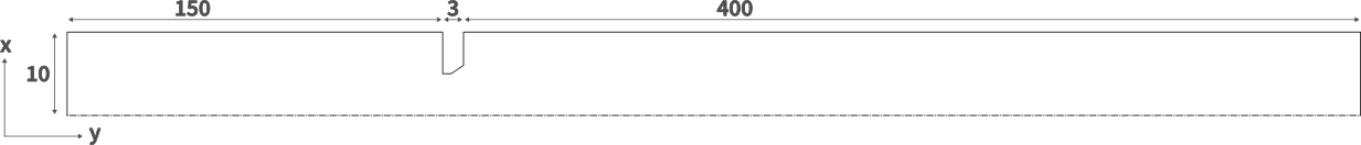
A schematic of half the orifice plate is shown above. The distances are shown in millimeters. Only half the orifice plate is modeled, as it is going to be modeled as axisymmetric around the center line, shown as dot dashes. Not to scale.
Time to complete: 40 minutes.
Pre-requisite tutorials: Ansys Workbench Familiarisation
Software version: This tutorial was prepared using Ansys 2024 R1. There may be minor differences when following the tutorial on later versions.
Before starting this tutorial:
Step 1: Open the project file. From the Workbench interface, open the downloaded project file by selecting File and then Open from the top menu. Navigate to where the project files is, select it and click Open. The Project Schematic should now display a Geometry System as A connected to a Mesh System as B.
Step 2: Add a Fluent system. Expand the Components System menu from the Toolbox and drag a Fluent component system onto the third row of Mesh system B, as shown below.
Step 2b: Update the project if needed. If a lightning strike appears in the Mesh system, this implies that the connection between the Mesh system and the Fluent system needs updating. This can be done using the Update Project button on the top menu. You may need to wait a while for this to process and it may end with an error message stating "Update failed for the Solution component in Fluent. Update solution Failed". Do not worry about this – it is attempting to populate the project files with results from a CFD calculation that has not been conducted yet. Just press OK. If the firewall dialogue box appears, this can usually be dismissed with the "Cancel" option, without causing any problems. You may need to do this several times.
Step 3: Open Fluent. Double Click the Setup cell in Row 2 of the Fluent System C. This will open the Fluent Launcher window. Click Setup or Start to open the Fluent software. This may take a moment to read in the data and display the interface.
In the Fluent Launcher window, we were presented with a few options. One was to select either a 2D or 3D simulation. In this case, the mesh has been connected to the Fluent system in the Workbench, so it knows the incoming mesh is 2D and this option is selected and the ability to change it is greyed out. There is also an option to select the number of processes across which the simulations should be parallelized. For large meshes, it can be faster to distribute the calculation across multiple processes if you have them in your computer. In this case, our mesh is small, and so we will accept whatever has been chosen by default.
Step 4: Check the mesh. Double Click General in the Outline View to open the General options in the Task Page. It is sensible to run a check on all incoming meshes to see if any errors are detected. Under the Mesh options of the Task Page, click Check. A series of data about the mesh will appear in the Console, and if all the checks are passed, this will terminate with the word Done.
Step 5: Apply axisymmetric model. Still within the General Task Page, Under the Solver and 2D space options, select Axisymmetric.
The Axisymmetric model will calculate the simulation on the 2D mesh assuming that it represents a slice of a 3D object that would be created if the slice were rotated 360 degrees around the x-axis. The code has no option to specify the axis of rotation, it always uses the positive x-axis. Axisymmetric meshes must be built with this in mind.
In the next step, we are going to apply a viscous model to account for turbulence in the simulation. Before proceeding, you should determine if the flow is turbulent. Calculate the Reynolds number for the inlet, using a velocity of 1 m/s, a diameter of 20 mm, and the material properties of water. Is this above the critical Reynolds number of 2,300 for internal flow?
Step 6: Apply a turbulence model. Expand the Models menu from the Outline View. Double click Viscous (SST k-omega) to open the Viscous Model options page. Under the Model options, ensure SST k-omega is selected. Click OK.
The "Viscous Model" page allows you to specify how turbulence is simulated. It is possible to run an inviscid simulation, with no friction, or a laminar simulation, where there is no turbulence. However, if your simulation requires turbulence (because the Reynolds number has exceeded the critical value) , one of several different models needs to be chosen. In this case, we are going to use the k-omega model, which adds two more conservation equations and creates two variables in each cell to store values to account for the turbulence.
Step 7: Input material properties. Expand the Materials menu from the Outline View, and then expand the Fluid menu, to reveal the default material, "air". Double click air to bring up the properties of this material. Under Name, change the word from "air" to "water". If you want to add a Chemical Formula of "h2o", feel free. Under the Properties menu, input a density value of 1000 (this will be in kilograms per meter cubed) and a viscosity value of 0.001 (this will be in Pascal seconds). Click Change/Create and this will bring up a window asking if you want to Overwrite air. Click No. Close the material properties window.
When the material "water" was added to the material's list, this did not specify to which parts of the domain it will apply. It may seem obvious, as there is only one material across the whole domain of this simulation. But because the software is capable of simulations where different materials exist in different locations, for example mixing or chemical reactions, the users must specific which materials are applied to which sections. In the Materials menu of the tree outline, it is possible to build a list of materials that will be used in the simulation. In the next step we will instruct the software which materials to apply to which cells of the mesh.
Step 8: Add cell zone conditions. Expand the Cell Zone from the Outline View, and then expand the Fluid menu, to reveal the surface, "solid-surface_body". Double click solid-surface_body to bring up the Zone Names properties for this surface. From the Material Name drop down menu, select water (or whatever name you gave it in the previous step). Click Apply and then Close.
In the next step we will apply boundary conditions to any mesh elements at the edge of the domain. These are the boundary conditions the software needs to solve the governing equations. There needs to be a condition for every variable that is being solved for, in this case x-velocity, y-velocity, pressure and two variables to account for turbulence (k and omega), on every boundary surface. However, the Fluent software makes this process easier by allowing users to select physical boundary types, such as inlets, outlets, walls, and determining how to set the appropriate variables for each equation. Fluent attempts to select the correct boundary condition type based on the name provided in the Mesher. If the boundary is called something like "pipe inlet" it may guess that to apply a "velocity-inlet" boundary type. However, it can make decisions that might not have been your intention, so it is always good to check the boundary type that has been applied.
Step 9: Check boundary condition types. Double click Boundary Conditions in the Outline View and this will open the Boundary Conditions panel in the Task Page. Listed in the Task Page are previously named boundaries. Naming would typically happen during the meshing stage. In this case, these are Axis, Inlet, Outlet and Wall. There may be some internal surfaces, but as these are not on the boundary of the domain these do not need any conditions setting for them. Single click axis in the boundary conditions list and note the entry in the "Type" dropdown at the bottom of the Task Page. Ensure that Type is set to "axis" and if not, select this from the dropdown. Work your way down the list to check the following types:
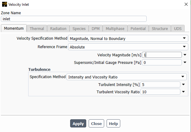
Step 10: Edit the boundary conditions. Double click inlet in the Task Page. This will bring up a window to allow you to edit the settings for the "Velocity Inlet" type boundary conditions. Input a value of 1 into the Velocity Magnitude [m/s] to set the inlet velocity magnitude to 1 meter per second. Make a note of the inlet velocity (you will need it later!). There is also the option to set the Turbulence boundary conditions in the Turbulence settings at the bottom of this window, but we will leave those at the default values, as they are reasonably representative in this case. Click Apply and then Close. The boundary conditions settings for the axis, outlet and wall can be accessed in the same way. While we will keep the default value for all of these, it is worth opening each one to check what settings are present. Interesting parts to note are that there is little you can set with an axis type boundary, the outlet pressure is set to 0 Pa, gauge, and the wall has a no-slip shear condition.
In the next step we will initialize the calculation. As the calculation is an iterative, numerical method that updates the solutions based on a previous prediction, initial values are required. Values of every solution variable are required for every mesh element. Fortunately, there are tools built into the Fluent software to make this process easier.
Step 11: Initialization. Expand the Solution menu from the Tree Outline. Double click Initialization. In the Task Page, Under Solution Initialization, select Standard Initialization. In the Compute from dropdown, select inlet and all the values specified in the inlet boundary conditions will appear below under Initial Values. Click the Initialize button.
In Fluent, there are two common options for initialisation, "Standard" or "Hybrid". In "Standard", you can specify values for each of the solution variables. The software will apply these values to all of the mesh elements. You can also call the values from each of the solution variable from any of the boundary conditions you have previously set up. In this case, because the flow along the length of the tube will be broadly like the conditions at the inlet, this is what we have chosen to do. Of course, the flow will be faster than the inlet at the throat of the orifice plate, and will slow down at the wall due to friction, but as this is just an initial guess to start the iterative calculation, it is a reasonably good starting point.
Step 12: Run the calculation. Within Solution in the Tree menu, double click Run Calculation. In the Task Page, under Parameters, enter 1000 in the Number of Iterations text entry box. Click Calculate. You should see the residuals appear in the Graphics window.
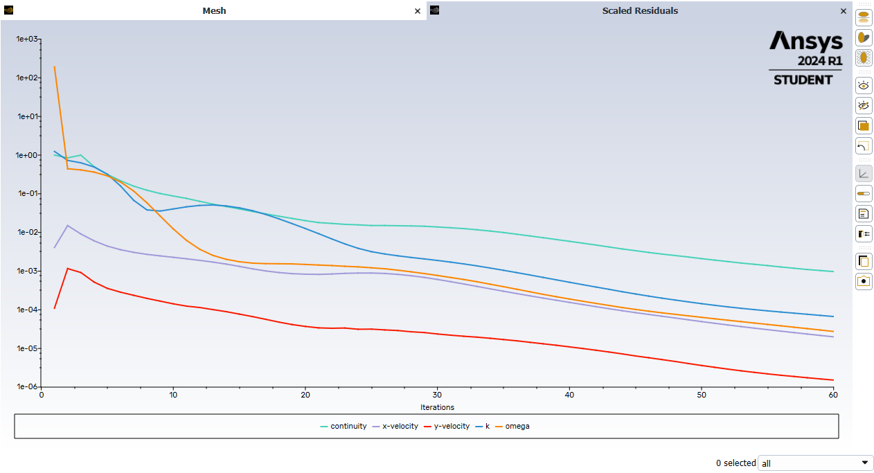
When selecting the number of iterations, in this case 1000, this is the maximum number of iterative calculations the software will perform. The software will stop calculating if the convergence criteria are reached before it has reached the maximum number of iterations. The default convergence criteria are set to all solutions variable reaching a residual value of 0.001. If you want to make the convergence criteria more strict, this can be set from the Monitors then Residuals option on the left hand menu. The values of Absolute Criteria could be reduced, for example to 0.0001, and the calculation continued (using the method in step 12) to produce a more precise solution. This is not necessary for this exercise.
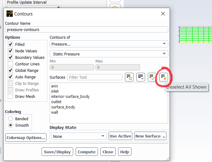
Step 13: Produce a pressure contour plot. In this step we will generate an image to show the distribution of pressure in the domain. Expand the Results and Graphics items on the Tree menu. Double click Contours to bring up Contours window. In the Contour Name box, enter the name "pressure-contours". Under Contours of, the default of Pressure and Static pressure should be selected. If not, select these from the drop down. Finally, deselect everything in the Surfaces list, by clicking the Deselect All Shown button or just clicking each surface one by one. Click the Save/Display button.
The window should display the pressure contours calculated inside the orifice plate, similar (but not necessarily identical) to the image above. If you can't see the picture, it might be because you need to select the tab at the top of the graphics window that says "Contours of Static Pressure [Pa]". You can also select the Scaled Residuals from the other tab. In the image above, the red colour indicates high pressure, as illustrated on the scale to the left. As the flow accelerates, the pressure drops, and the colour moves down the scale. In this simulation, the pressure is around 6,000 or 7,000 Pa, at the inlet, and drops to about -4,000 or -5,000 Pa at the throat, which is a 10-12 kPa pressure drop.
Step 14: Produce a velocity contour plot. In this step we will generate an image to show the distribution of velocity in the domain. Double click the Contours item from the tree menu again to bring up the Contours window. In the Contour Name box, enter the name "velocity-contours". Under Contours of, change the default to Velocity and Velocity Magnitude. Deselect everything in the Surfaces list, by clicking the Deselect All Shown button and click the Save/Display button.
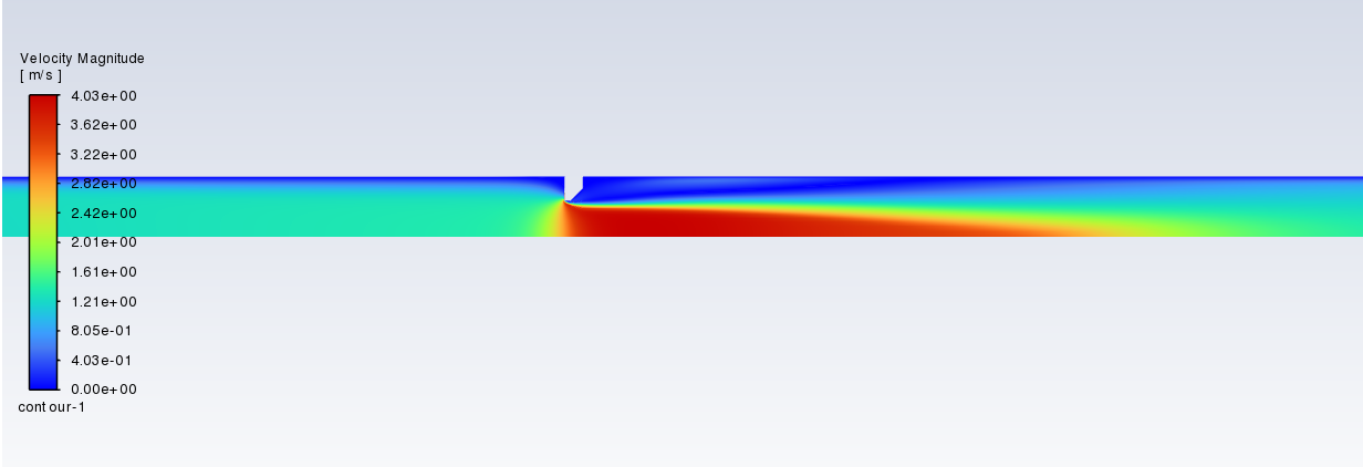
The window should display the velocity contours in the Graphics window, with a scale in m/s to the left. You should be able to see the fluid accelerating as the diameter reduces at the throat.
Step 15: Produce a graph of pressure. In this step we will generate a graph of the pressure distribution along the axis. Expand the Results and Plots items on the Tree menu. Double click XY Plot to bring up Solution XY Plot window. Under XY Plot Name enter "axis-pressure". Leave the Plot Direction as X=1, Y=0, as the axis is in the positive X direction. Ensure the Default Y Axis Function is the default value of Pressure and Static Pressure. Finally, select the axis from the list of surfaces. Click the Save/Plot button and the graph of static pressure along the axis should appear in the Graphics window.
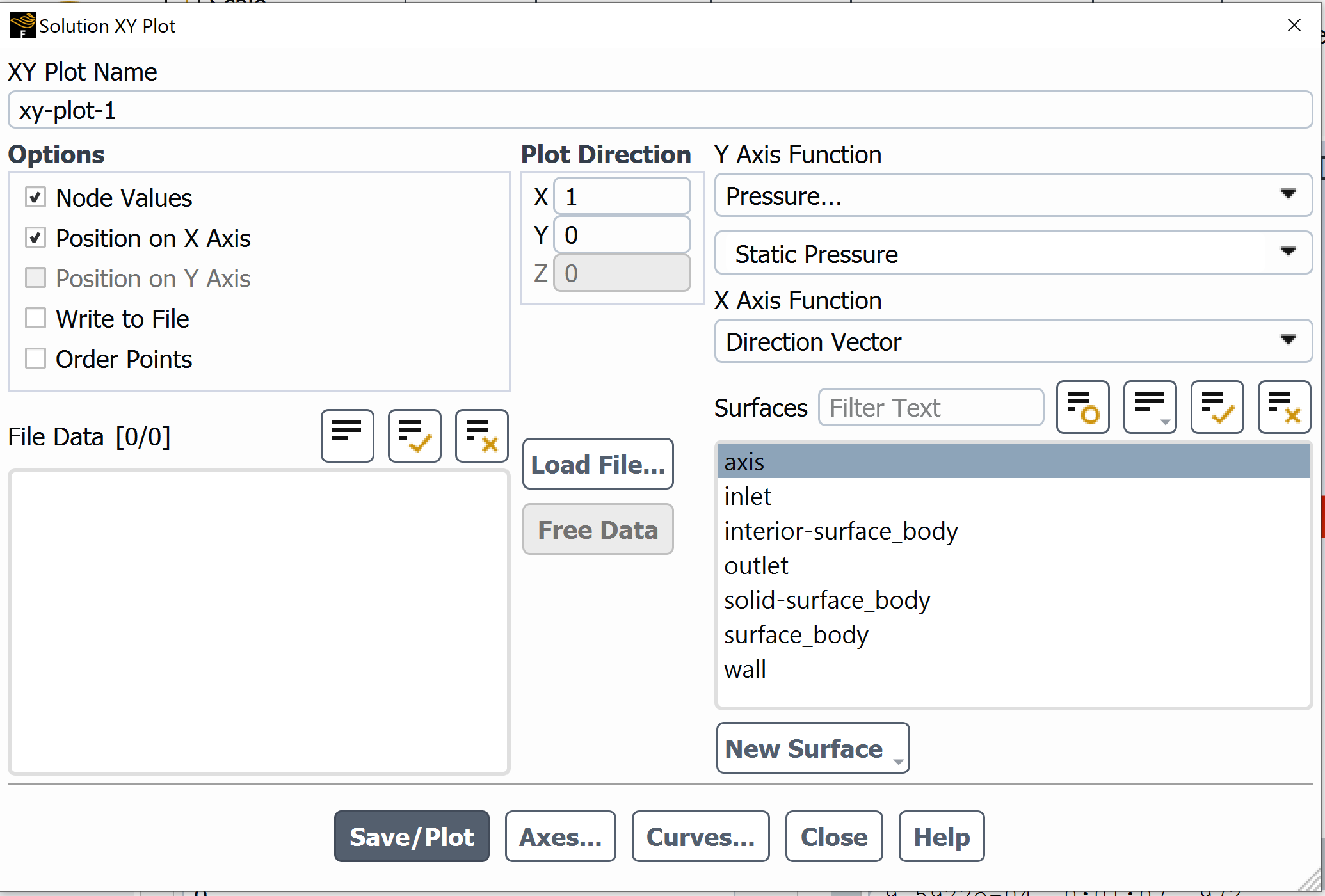
Step 16: Produce a graph of velocity. In this step we will generate a graph of the velocity distribution along the axis. Return to the Solution XY Plot window. Under XY Plot Name enter "axis-velocity". Change the Default Y Axis Function to Velocity and Velocity Magnitude. Select the axis from the list of surfaces. Click the Save/Plot button and the graph of velocity magnitude along the axis should appear in the Graphics window.
While not necessary at this stage, as the simulation is over, it is a good habit to get into saving your work as you go along. This can be done from the File menu at the top, and selecting Save Project.
Use the results from postprocessing the simulation to find the coefficient of discharge for the orifice plate. This is defined as the actual flow rate over the theoretical flow rate (measured using the pressure drop predicted by Bernoulli).In these steps, you will not be using the Ansys software. You will be extracting values calculated by the software in order to validate the result.
Step 17: Calculate the actual flow rate. Use the inlet velocity set in the inlet boundary condition panel, and multiply this by the inlet area (the diameter is 20 mm). This will give you the actual inlet flow rate in units of cubic meters per second.
Step 18: Calculate the theoretical flow rate. Use the pressure along the axis graph to determine the change of pressure between the inlet and throat of the orifice plate. With the pressure drop and the areas of the inlet and orifice constriction, calculate the flow rate predicted by Bernoulli (assuming no friction, which is why it is theoretical), using the equation below, where Q is flowrate, P is pressure, rho is the denity, A1 is the area at the inlet and A2 is the area at the throat.
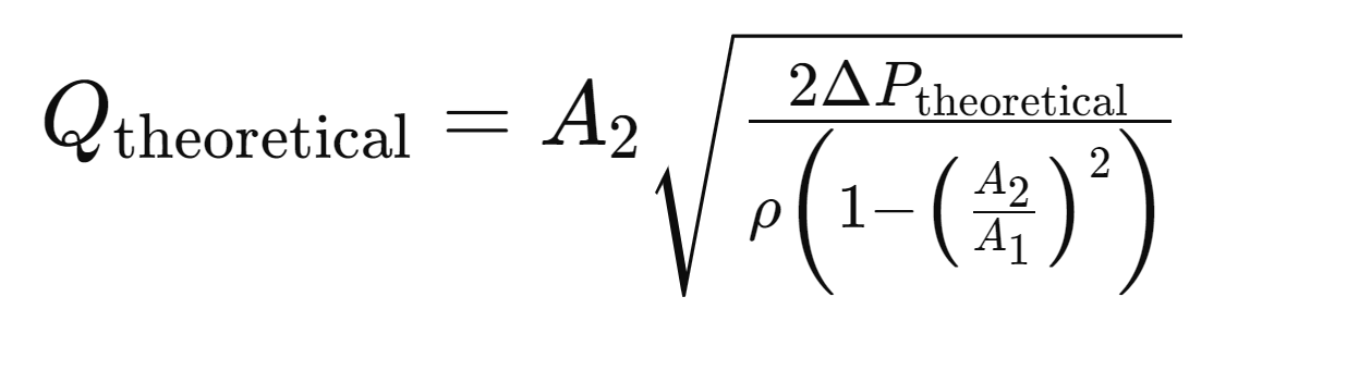
Step 19: Calculate the coefficient of discharge for the orifice plate. Divide the actual flow rate (known because we know the inlet velocity and inlet area) by the theoretical flow rate (predicted by Bernoulli assuming no friction). Do you know the coefficient of discharge for a standard orifice plate?
Now you are able to preprocess the simulation of the simulation and validate the solution with theory, consider attempting to adjust the parameters of the simulation. Can you repeat this with different inlet velocities (2, 5 or 10 m/s for example). What about using a different fluid, such as air? Remember! When you make changes to the simulation parameters, you will need to repeat the initialisation and run the calculation again before the results stored in the computer will change.
Congratulations on reaching the end of this tutorial. In summary, you have learned to: