In this tutorial, we will use the Ansys Fluent software to open a "workbench" file which contains three 3D simulations of different shapes of bottle rocket nose cones. The aim of the exercise is to determine the coefficient of drag for each configuration. The three bottle rockets are a cylinder, the same cylinder with a cone at the leading edge, and the same cylinder with a hemisphere on the leading edge. The cylinder is 300 mm long and 110 mm in diameter. The domain surrounding the bottle rockets is filled with air and is 2 meters in length and 0.5 meters in diameter. In the simulation, we will set the material to air, set the boundary conditions for the inlet, outlet, bottle rocket, and the surrounding cylinder, and calculate a full CFD solution. From this, we will extract contour plots of pressure and velocity, as well as extract a numerical value for drag in Newtons. From the drag force value, we can calculate the coefficient of drag.
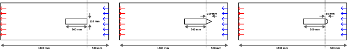
A schematic of the bottle rocket is shown above. A slice through the centerline of the 3D shape is shown. Not to scale.
Time to complete: 40 minutes.
Pre-requisite tutorials: Ansys Workbench Familiarisation
Software version: This tutorial was prepared using Ansys 2023 R2. There may be minor differences is following the tutorial on later versions.
Before starting this tutorial:
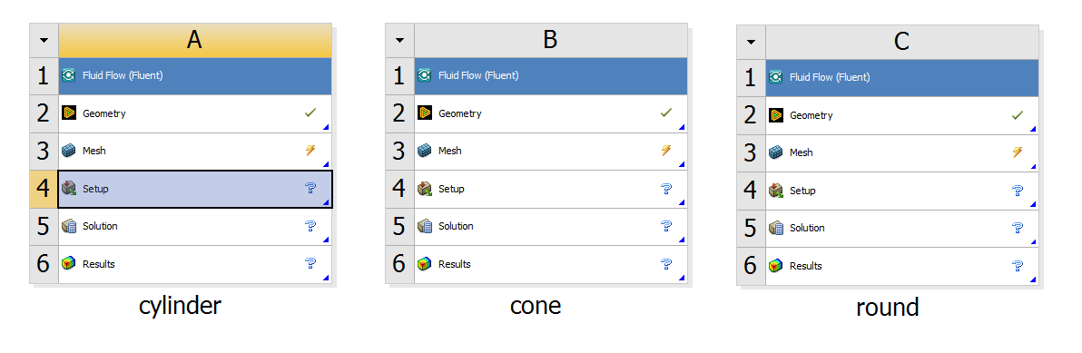
Step 1: Open the project file. From the Workbench interface, open the downloaded project file by selecting File and then Open from the top menu. Navigate to where the project file is, select it, and click Open. The Project Schematic should now display three systems: A for the cylinder, B for the cone, and C for the rounded bottle rocket.
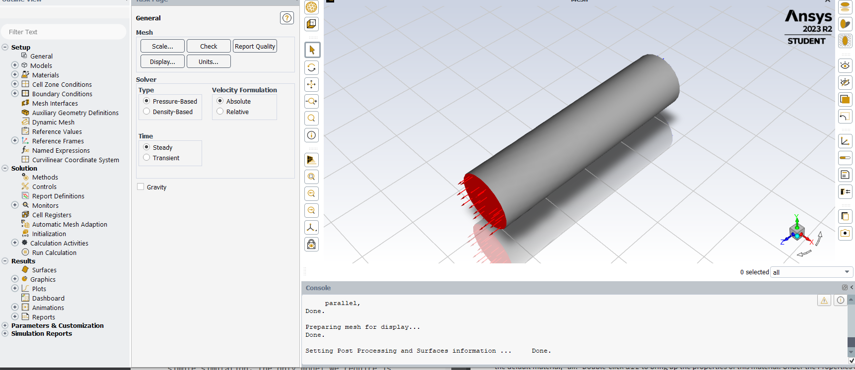
Step 2: Open Fluent system for Cylinder. Double-click Setup on the 4th row of the Cylinder A component on the project schematic. This will open the Fluent Launcher window. Click Setup or Start to open the Fluent software. This may take a moment to read in the data and display the interface. Dismiss any update messages displayed in the Fluent window by clicking OK.
In the Fluent Launcher window, we are presented with a few options. One is to select either a 2D or 3D simulation. In this case, the mesh has been connected to the Fluent system in the Workbench, so it knows the incoming mesh is 3D; this option is selected and the ability to change it is greyed out. There is also an option to select the number of processes across which the simulations can be parallelized. For large meshes, it can be faster to distribute the calculation across multiple processes if you have them in your computer. In this case, our mesh is small, so we will accept whatever has been chosen by default.
Step 3: Check the mesh. Double-click General in the Outline View to open the General options in the Task Page. It is sensible to run a check on all incoming meshes to see if any errors are detected. Under the Mesh options of the Task Page, click Check. A series of data about the mesh will appear in the Console, and if all the checks are passed, this will terminate with the word Done.
Step 4: Check the models. From the Outline View on the left, double-click Models to expand this menu item. Ensure the Viscous Model is set to capture turbulence, with a model such as (SST k-omega). All other models should be (OFF).
In this section of the Fluent software, you can add models to capture various aspects of physics you may want to use in your simulation. For example, heat, chemical reactions, or multiple phases (both liquids and gases) can be set up here. In this simple simulation, the only model we require is turbulence, which is on by default.
The "Viscous Model" page allows you to specify how turbulence is simulated. It is possible to run an inviscid simulation, with no friction, or a laminar simulation, where there is no turbulence. However, if your simulation requires turbulence (because the Reynolds number has exceeded the critical value) , one of several different models needs to be chosen. In this case, we are going to use the k-omega model, which adds two more conservation equations and creates two variables in each cell to store values to account for the turbulence.
Step 5: Check material properties. Expand the Materials menu from the Outline View, and then expand the Fluid menu to reveal the default material, "air." Double-click air to bring up the properties of this material. Under the Properties menu, note the value of density and viscosity (you will need this later!). We may need to use these later. Click Close. Close the material properties window.
In this part of the software, we can, if required, change the properties of air or create new materials. Our simulation is of a bottle rocket travelling through air, so we can accept the default material and material properties. You can update them if you want to change them.
In the next step we will apply boundary conditions to any mesh elements at the edge of the domain. These are the boundary conditions the software needs to solve the governing equations. There needs to be a condition for every variable that is being solved for, in this case x-velocity, y-velocity, z-velocity, pressure and two variables to account for turbulence (k and omega), on every boundary surface. However, the Fluent software makes this process easier by allowing users to select physical boundary types, such as inlets, outlets and walls, then determining how to set the appropriate variables for each equation. Fluent attempts to select the correct boundary condition type based on the name given to the surface. If the surface is called something like "pipe inlet" it may guess that it should to apply a "velocity-inlet" boundary type. However, it can make decisions that might not have been your intention, so it is always good to check the boundary type that has been applied.
Step 6: Check boundary condition types. Double-click Boundary Conditions in the Outline View to open the Boundary Conditions panel in the Task Page. Listed in the Task Page are named surfaces. In this case, these are "bottle," which is the surface of the bottle in the center of the domain, "inlet" where air is entering the domain, "outlet" where air can leave the domain, and "surround," which is the cylinder surrounding the domain. There may be some internal surfaces, but as these are not on the boundary of the domain, they do not need any conditions set for them. Single-click bottle in the boundary conditions list and note the entry in the "Type" dropdown at the bottom of the Task Page. Ensure that the Type is set to "Wall" and if not, select this from the dropdown. If any dialogue boxes appear inviting you to edit properties of the boundary, close these as we will work on them in the next section. Work your way down the list to check the following types:
Step 7: Edit the inlet boundary conditions. Double-click inlet in the Task Page. This will bring up a window to allow you to edit the settings for the "velocity-inlet" type boundary conditions. Input a value of 10 into the Velocity Magnitude [m/s] to set the inlet velocity magnitude to 10 meters per second. Note the value of velocity input (you will need this later!) There is also the option to set the Turbulence boundary conditions in the Turbulence settings at the bottom of this window under Turbulence. You can change how to specify turbulence at an inlet boundary by setting the Specification Method. In this case, we will set the specification method to "Intensity and Hydraulic Diameter." Input the Turbulent Intensity to 5% and the Hydraulic Diameter to 0.11 m. Click Apply and then Close.
Step 8: Edit the surround boundary conditions. As you did with the inlet, double-click surround in the Task Page. This will bring up a window to allow you to edit the settings for the "wall" type boundary conditions. This surface is not a solid wall. It is a surface sufficiently far from the air around the bottle rocket to not influence the flow around the bottle rocket. If it were a solid wall, it would have a "no-slip" boundary condition. As this is not a solid wall, it will need a "slip" boundary condition. Under "Shear Condition," select Specified Shear and leave all the X, Y, and Z components as zero Pascals. Click Apply and then Close.
Step 9: Check the other boundary conditions. The default values for the outlet and bottle (wall) boundaries should be appropriate for our simulation, but it is a good idea to check. Double-click outlet in the Task Page. This will bring up a window to allow you to edit the settings for the "pressure-outlet" type boundary conditions. Ensure that the "Gauge Pressure" is set to 0 Pa and close the window. Double-click bottle in the Task Page. Ensure "Stationary Wall" and "No Slip" are selected, and close the window.
In the next step, we will initialize the calculation. As the calculation is an iterative, numerical method that updates the solutions based on a previous prediction, initial values are required. Values of every solution variable are required for every mesh element. Fortunately, there are tools built into the Fluent software to make this process easier.
Step 10: Initialization. Expand the "Solution" menu from the Tree Outline. Double-click Initialization. In the Task Page, under Solution Initialization, select Standard Initialization. In the "Compute from" dropdown, select inlet, and all the values specified in the inlet boundary conditions will appear below under Initial Values. Click the Initialize button.
In Fluent, there are two common options for initialization: "Standard" or "Hybrid." In "Standard," you can specify values for each of the solution variables. The software will apply these values to all of the mesh elements. You can also call the values for each of the solution variables from any of the boundary conditions you have previously set up. In this case, because the flow along the length of the domain will be broadly like the conditions at the inlet, this is what we have chosen to do. Of course, the flow will be faster than the inlet at the throat of the venturi and will slow down at the wall due to friction. As this is just an initial guess to start the iterative calculation, it is a reasonably good starting point.
Step 11: Run the calculation. Under "Solution" in the Tree menu, double-click Run Calculation. In the Task Page, under Parameters, enter 100 in the "Number of Iterations" text entry box. Click Calculate. You should see the residuals appear in the Graphics window.
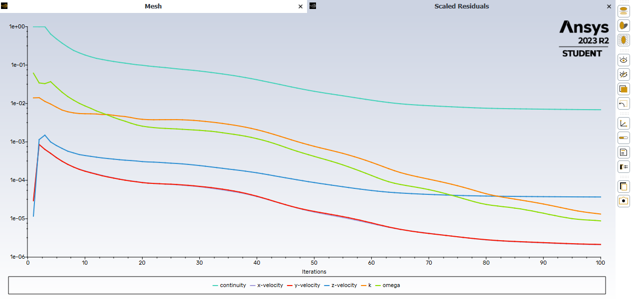
The residuals should drop as the calculation progresses. When selecting the number of iterations, in this case 100, this is the maximum number of iterative calculations the software will perform. The software will stop calculating if the convergence criteria are reached before it has reached the maximum number of iterations. In the case shown below, the convergence has reached a value of 0.006 and stopped at 100 iterations. Do not worry if your output is slightly different from this.
In this section, we will create a graphical plot to show the flow around the bottle rocket and calculate the drag. Because the simulation is 3D, we will need to create a plane through the domain in order to show the results.
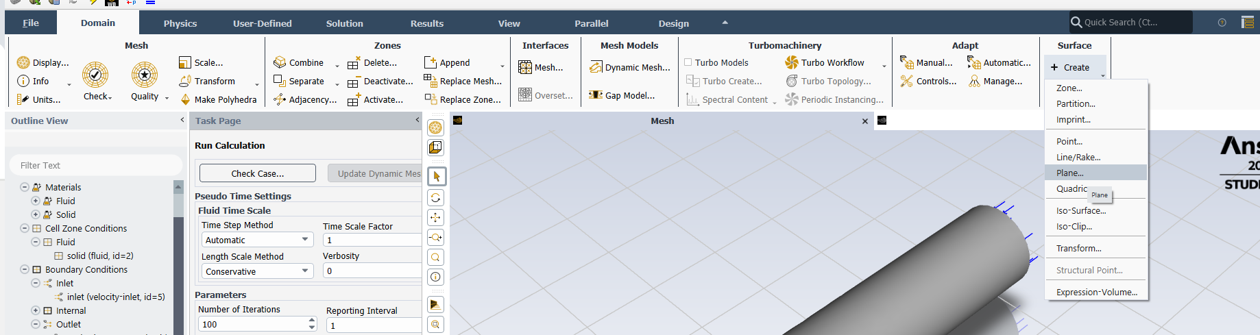
Step 12: Create a plane. Using the menus at the top of the Ansys Fluent window, select "Domain" and "Surface." Select "Plane" from the "Create" dropdown. The "Plane Surface" window should appear. Here, you can name the plane (or just make a note of the default name) and specify the method to create the plane. In our domain, the flow is in the Z direction, so we are going to create a plane in ZX. Under "Method," select ZX Plane and under "Y" distance set the value to 0 m. Click Create and Close the window.
Step 13: Produce a pressure contour plot. In this step, we will generate an image to show the distribution of pressure in the domain. Expand the Results and Graphics items on the Tree menu. Double-click Contours to bring up the Contours window. In the "Contour Name" box, enter the name pressure-contours". Under "Contours of," the default of Pressure and Static pressure should be selected. If not, select these from the dropdown. Finally, deselect everything in the "Surfaces" list by clicking the "Deselect All Shown" button or deselecting them one by one. Select the newly created plane, with the name given or noted from the previous step. Click the Save/Display button. The pressure contour plot should be displayed in the graphics window.
Step 14: Produce a velocity contour plot. Repeat the process from the previous step but change the "Contour Name" to velocity-contours" and under "Contours of," select Velocity and Velocity Magnitude from the dropdown menus. Click the Save/Display button. The velocity contour plot should be displayed in the graphics window.
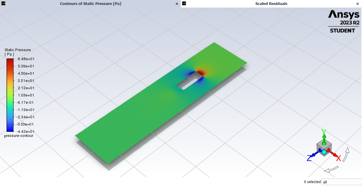
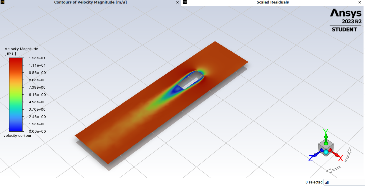
The window should display the pressure and velocity contours around the bottle rocket, similar (but not necessarily identical) to the image above. If you can't see the picture, it might be because you need to select the tab at the top of the graphics window that says "Contours of Static Pressure [Pa]." You can also select the Scaled Residuals from the other tab. In the image above, the red color indicates high values and blue indicates low values, as illustrated on the scale to the left. Is this what you expected?
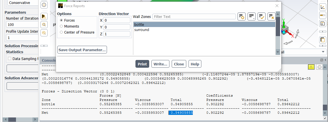
Step 15: Calculate drag. Expand the Results and Reports items on the Tree menu. Double-click Forces to bring up the "Force Reports" window. We want the drag from the bottle rocket, which is aligned in the Z direction. Under "Direction Vector," set X to 0, Y to 0, and Z to 1. Under "Wall Zones," ensure only "bottle" is selected. Click Print. In the Console of the Fluent interface, the total force is reported in Newtons. Note the value of force (you will need this later!)
Lots of details from the force calculation are shown in the Console. For each surface selected, the Pressure and Viscous forces will be shown. In the case of drag, this would be the form and skin friction drag, respectively. The total is the sum of these two forces. In this case, the Viscous drag is effectively negligible. You may also see the "Coefficients" displayed. Do not assume these are correct. In order to calculate the drag coefficient, Fluent would require a reference area, which is set in another part of the software. The calculation of the drag coefficient can be done manually (or in another piece of software) using the value of the projected area of the bottle rocket.
While not necessary at this stage, as the simulation is over, it is a good habit to get into saving your work as you go along. This can be done from the File menu at the top, and selecting Save Project.
Use the results from postprocessing the simulation to find the coeffient of drag.
Step 16: Calculate drag coeffieient. Using the formula below (from Wikipedia) calculate the Coefficient of Drag. Use the Density from the Materials panel and the Velocity from the velocity-inlet boundary conditions panel of fluent. The area in th equation is the projected area of the cylinder, of diamter 110 mm. The force is the value reported in the Fluent Console.

The simulation can be repeated on the cylinder at different velocities. You must remember to reinitalize and rerun the calculation every time a change is made to the simulation parameters. Will the coefficient of dischange change with velocity?
Exactly the same procedure can be applied to the cone and rounded
Congratulations on reaching the end of this tutorial. In summary, you have learned to: