---
title: "Pretty Convincing?"
subtitle: "My Opinionated Introduction to CFD"
kicker: "MEC Lecture · Computational Fluid Dynamics"
author: "Professor Andrew Garrard MEng(hons) PhD CEng FIMechE PFHEA"
details: "MAC118"
date: "2026-08-08"
theme: "white"
base: "../../../"
---     

## What we will learn today

<!-- "G:\My Drive\Teaching\framework\convert.bat" "G:\My Drive\Teaching\teaching-presentations\cfd\Pretty convincing\prettyConvincing.md" -->

::: {.learning-outcomes}
By the end of this lecture you will be able to:
1. Outline how CFD developed into its current state of the art
2. Explain why and how CFD is used alongside experiment and theory
3. Describe the steps involved in simulating a fluid flow numerically
4. Relate broad CFD concepts to the applications in the tutorials
:::

# Introduction

## CFD stands for
* <b>C</b> - Computational
* <b>F</b> - Fluid
* <b>D</b> - Dynamics

> Computational fluid dynamics (CFD) is a branch of both fluid mechanics and computational physics that uses numerical analysis and data structures to analyze and solve problems that involve flows.
>
> — [Wikipedia, "Computational fluid dynamics"](https://en.wikipedia.org/wiki/Computational_fluid_dynamics)

. . .

::: {.fragment}
_Alternatively_

> Colours for Directors
:::


::: {.fragment}
_a.k.a_

> "The Beautiful Lie"

:::

## Contemporary uses of CFD

A simulation to determine safety for Urban Air Mobility.

![A single two-bladed rotor hovering above a grey ground plane, surrounded by a dense tangle of thin blue vortex tubes that spread out across the ground, with brighter green and magenta rings trailing just below the rotor tips.](https://www.nas.nasa.gov/assets/nas/images/content/stories/06_Ventura_P_UAM_ground_med.jpg)
: Hovering quadcopter rotor in ground effect. Image: Patricia Ventura Diaz and D-G Caprace, Tim Sandstrom. NASA/Ames.

<!-- The link opens in a new tab so the deck stays where it is; close the tab to come back. The animation on that page is credited to Tim Sandstrom, NASA/Ames. -->

<a href="https://www.nas.nasa.gov/pubs/stories/2024/feature_simulations_for_urban_air_mobility_safety.html" target="_blank" rel="noopener">Watch the simulations on the NASA page</a>

<!-- This link shows flow visualization of NASA’s quadcopter isolated rotor hovering in ground effect, with the ground located at one rotor radius below the rotor. Isosurfaces colored with the vorticity magnitude show the vortex wake and the interactions with the ground, where purple is low and yellow is high. The flow visualization reveals the complex wake of a single rotor in ground effect.-->


# A history of CFD

## Fluid mechanics before computers

![Two separate circles, one labelled empirical and one labelled theory, with nothing between them.](/diagrams/cfd-history-1-separate.svg)
: From the 17th to the 19th century, fluid mechanics was split into two disciplines.

## Early CFD

![The same two circles, now overlapping, with CFD occupying the region where they meet.](/diagrams/cfd-history-2-overlap.svg)
: CFD arrives, and it is not well defined as either theory or experiment.

## A third way

![Empirical, theory and CFD as three circles, each joined to the other two by a double-headed arrow.](/diagrams/cfd-history-3-three-ways.svg)
: Three fields of fluid mechanics, of equal importance, each informing the others.

## Driving and bottlenecking CFD progress

![A log-scale chart of transistor counts per chip from 1970 to 2020, climbing in a near-straight line.](https://thumb.wikimedia.org/wikipedia/commons/thumb/0/00/Moore%27s_Law_Transistor_Count_1970-2020.png/1280px-Moore%27s_Law_Transistor_Count_1970-2020.png)
: Moore's law. Via Wikimedia Commons.

## Commercial computers

:::: {.columns}

::: {.column width="50%"}
![A Cray Y-MP supercomputer, a dark angular cabinet standing in a machine room.](https://thumb.wikimedia.org/wikipedia/commons/thumb/e/ec/Cray_Y-MP_GSFC.jpg/1280px-Cray_Y-MP_GSFC.jpg)
: A Cray Y-MP. ~1988: ~2.5 GFLOPS, ~20 million USD, ~55 million now USD. NASA Goddard, via Wikimedia Commons.
:::

::: {.column width="50%"}
![A Dell Latitude D630 laptop, open on a plain background.](https://thumb.wikimedia.org/wikipedia/commons/thumb/d/d3/Dell_Latitude_D630_8064.jpg/960px-Dell_Latitude_D630_8064.jpg)
: A Dell Latitude D630. Core 2 Duo PC, ~2008: ~25 GFLOPS, ~1,000 USD, ~1,500 USD now. Via Wikimedia Commons.
:::
::::
<!--
Intel Core i7-1260P: ~500 GFLOPS.
-->


## Pushing boundaries in fluid mechanics

<!-- The X-59 took its first flight in the morning of October 28, 2025, from Air Force Plant 42, and landed around an hour later at NASA's Armstrong Flight Research Center in Edwards Air Force Base. The aircraft remained subsonic for this initial flight, reportedly reaching 230 mph at an altitude of 12,000 feet.[26] On April 3, 2026 the X-59 completed its first wheels up flight, reaching 20,000 feet and approximately 460 mph.[27] On June 5, 2026, the X-59 went supersonic to approximately Mach 1.1 for the first time.[28][29] One week later, it reached Mach 1.4.[30] -->

![A slender dart-shaped vehicle streaking through high cloud, its leading edges glowing orange with the heat of the airflow.](/images/LockheedMartinHypersonic.jpg)
: A Lockheed Martin hypersonic vehicle.

## Pushing boundaries in fluid mechanics

![A flow visualization of NASA’s X‑59 supersonic, low-boom aircraft concept.](https://nas.nasa.gov/assets/nas/images/content/stories/feature_jensen_lowboom_big.png)
: A flow visualization of NASA’s X‑59 supersonic, low-boom aircraft concept. This computational fluid dynamics simulation, produced on the Pleiades supercomputer using the NAS-developed Launch Ascent and Vehicle Aerodynamics (LAVA) code, will be used to help determine which components contribute to the pressure signatures below the aircraft that create the sonic boom in flight. Red and blue represent high and low pressure, respectively; the symmetry plane—which bisects the vehicle along its center line—is colored by Mach number. James Jensen, NASA/Ames.

[https://nas.nasa.gov/pubs/stories/2021/feature_X-59.html](https://nas.nasa.gov/pubs/stories/2021/feature_X-59.html)


<!-- Before its decommissioning in January 2026, it was ranked the 218th most powerful computer on the TOP500 list with a LINPACK rating of 5.95 petaflops (5.95 quadrillion floating point operations per second)[2] and a peak performance of 7.09 petaflops from its most recent hardware upgrade.[4] The system served as NASA's largest supercomputing resource, supporting missions in aeronautics, human spaceflight, astrophysics, and Earth science. -->

## Wind tunnels
The most powerful wind tunnel in the world.

![The JF-22 hypersonic wind tunnel at the Chinese Academy of Aerodynamics. Pandaily, https://pandaily.com/jf22-hypersonic-wind-tunnel-10km-jul2026, obtained 2026-09-11.](/images/jf22.png)

## A couple of issues with wind tunnels

:::: {.columns}

::: {.column width="50%"}
### Power

The JF-22 uses 15 GW of power.

. . .

![A Rolls-Royce Trent XWB turbofan, cut away along its length.](/images/TrentXWBengine.png)
: 180 × Trent XWB engines.

![Iron Man in flight in his red and gold armour.](/images/Iron_Man.png)
: 5 × Iron Men.
:::

::: {.column width="50%"}

. . . 

### Scale

The JF-22 has a working section of 4 m.

Real planes are bigger than 4 m across.

$$Re = \frac{\rho V L}{\mu}$$

. . .

The run time is less than 120 ms.
:::

::::

## Why use CFD?

* Cheaper
* Safer
* Unphysical problems
* Complete dataset
* Data after experiment
* Increasingly automated 

. . . 
::: {.fragment}
_But..._
* No exact solution
* No idea if the answer is correct – "black box engineering"
* Good for some situations, not for others - this requires some wisdom
:::

. . . 
::: {.fragment}
_Why I like CFD_
* I can work independently
* Easy "what if" scenarios
* Work from anywhere
:::

## Numerical experiment
CFD can be a portable, cheap wind tunnel.

> Numerical experiment

* Used to test a model, theory or hypothesis.
* Fewer factors are outside your control than in a physical experiment, but not none.
* Error will occur and has to be understood and accounted for.
* Good experimental design needs to be performed before starting.
* Experiments should adhere to the scientific method.
* Focus should always be maintained on the reasons for conducting the experiment.

## Something for everyone

![Seven stacked bars from engineering application at the top down to hardware.](/diagrams/cfd-stack.svg)
: The CFD stack: every answer rests on six layers the engineer never sees.

<!-- -->

## Some of my work
* Simulation of a "personal cloud"
* Prediction of smoke ingress and movement in offshore installations
* GRP spraying of boat hulls
* Electric motor cooling
* Fuel cell electrochemical modelling

:::: {.columns}

::: {.column width="50%"}
![Cutaway of a motor with coloured streamlines through the windings and velocity vectors fanning past the rotor poles.](/images/cfd_motor_AG.jpeg)
: Cooling and windage loss in a switched reluctance motor.
:::

::: {.column width="50%"}
![Three stages side by side: a bare cylindrical manifold, streamlines spiralling along it, then a dense vector field.](/images/fuel_cell_mainfold_AG.jpg)
: Swirl in a fuel cell stack manifold.
:::

::::

## Commercial software

:::: {.columns}

::: {.column width="50%"}
### In the recent past
Dedicated CFD platforms
* Fluent
* CFX
* STAR-CD
* COMSOL (general)
* OpenFOAM (open source)
:::
. . . 

::: {.column width="50%"}
### Now
Large multiphysics packages
* Ansys (Synopsys)
* Dassault Systèmes
* CAD bolt-ons (not very good)
* COMSOL (general)
* OpenFOAM (open source)
:::
::::
. . .

**At Sheffield we use Ansys Fluent.**

<!-- In 1979, Jim Swithenbank, at the time Professor of Chemical Engineering at the University of Sheffield, invited Boysan back to Sheffield to help him develop a code capable of interactively defining geometry and boundary conditions for a specific problem involving cyclone separators. The resulting software was developed with a student, Bill Ayers, as part of his final year research project and was published in the Transactions of the Institute of Chemical Engineers. With the permission of the authors, the editor of the publication added a note that readers could contact the authors to obtain a copy of the source code. Swithenbank and Boysan were surprised to receive several hundred requests for the code, alerting them to the commercial potential of an interactive CFD code. https://www.nafems.org/blog/posts/analysis-origins-fluent/?srsltid=AfmBOopakyIaFfFPIGLA3VZjCl19QUbzOLI8D3czKXd6mK8pdP1zOttu -->


## Fluent started in Sheffield

![A crowded, brightly coloured painting of Sheffield: Victorian buildings, a pub, a tram, a football match in the foreground, and the white Fluent offices flying international flags at the back.](/images/joe-scarborough-fluent.png)
: Joe Scarborough's painting of Fluent Europe's Sheffield, commissioned in 2000.

# How CFD works
From equations to numbers.


## The Navier–Stokes equations

Conservation of mass

$$\frac{\partial u}{\partial x} + \frac{\partial v}{\partial y} + \frac{\partial w}{\partial z} = 0$$

Conservation of momentum, in $x$, $y$ and $z$

$$\rho\left(\frac{\partial u}{\partial t} + u\frac{\partial u}{\partial x} + v\frac{\partial u}{\partial y} + w\frac{\partial u}{\partial z}\right) = -\frac{\partial p}{\partial x} + \mu\left(\frac{\partial^{2} u}{\partial x^{2}} + \frac{\partial^{2} u}{\partial y^{2}} + \frac{\partial^{2} u}{\partial z^{2}}\right) + \rho g_{x}$$

$$\rho\left(\frac{\partial v}{\partial t} + u\frac{\partial v}{\partial x} + v\frac{\partial v}{\partial y} + w\frac{\partial v}{\partial z}\right) = -\frac{\partial p}{\partial y} + \mu\left(\frac{\partial^{2} v}{\partial x^{2}} + \frac{\partial^{2} v}{\partial y^{2}} + \frac{\partial^{2} v}{\partial z^{2}}\right) + \rho g_{y}$$

$$\rho\left(\frac{\partial w}{\partial t} + u\frac{\partial w}{\partial x} + v\frac{\partial w}{\partial y} + w\frac{\partial w}{\partial z}\right) = -\frac{\partial p}{\partial z} + \mu\left(\frac{\partial^{2} w}{\partial x^{2}} + \frac{\partial^{2} w}{\partial y^{2}} + \frac{\partial^{2} w}{\partial z^{2}}\right) + \rho g_{z}$$

$u$, $v$, $w$ velocity components · $p$ pressure · $\rho$ density · $\mu$ dynamic viscosity

<!-- We solve the N–S equations. These look scary, but are actually very easy. They are conservation equations. -->

## Solving the Navier–Stokes equations

The Navier–Stokes equations cannot be solved analytically.

. . . 

::: {.fragment}
_Despite what Sam Altman says_

![Screen grab of BBC News from 8 September 2026, showing Sam Altman's face as the cover image and the headline "OpenAI says it cracked 90-year-old maths problem in 88 hours". https://www.bbc.co.uk/news/articles/cy7zygy3rl2o, 8 September 2026.](/images/OpenAI_solvesNS_08092026.jpg)
: OpenAI didn't solve the Navier–Stokes equations. From BBC News, https://www.bbc.co.uk/news/articles/cy7zygy3rl2o, 8 September 2026.
:::

## Basic conservation equation

:::: {.columns}

::: {.column width="50%"}
![A control volume drawn as a dashed blob, with an arrow bringing mass in across the boundary on the left and an arrow carrying mass out across it on the right, and the change of mass inside written in the middle.](/diagrams/conservation-1-mass.svg)
: Mass is conserved. The mass entering across the boundary minus the mass leaving across it is the mass accumulated inside.
:::

::: {.column width="50%"}
![The same control volume with momentum crossing the boundary in on the left and out on the right, three further arrows pressing inward on the boundary to represent forces, and the change of momentum inside written in the middle.](/diagrams/conservation-2-momentum.svg)
: Momentum is also conserved in the same way, but has a third route in: forces on the boundary.
:::

::::

## Discretising

::: {.demo src="/teaching-demos/cfd/cfd_cell_refinement.html" height="580" title="Mesh refinement demo"}
:::

<!-- Here’s a possible distribution that keeps the same total flow and slows down towards the walls. More cells let us represent that variation in more detail. The other equations of fluid motion decide what the actual distribution should be

One value at each cell. More cells means more refinement.
-->


## Typical CFD simulation workflow

![Eight green boxes in a column joined by downward arrows: create geometry, mesh geometry, define physics (energy, turbulence, species), define boundary conditions, define initial conditions, select solver and settings, run solver (and wait), post-process results.](/diagrams/cfd-workflow-1-pipeline.svg)
: The steps of running a CFD simulation.

## The more holistic CFD simulation workflow

![Six boxes in a column joined by downward arrows: determine the aim, determine the modelling strategy, actually do the CFD (the only green box), analyse the results, check the results are right, perform alternative tests. An arrow loops from the last box back up to the modelling strategy.](/diagrams/cfd-workflow-2-holistic.svg)
: Running the simulation is one step of six in a CFD study.

## The complete CFD simulation workflow

![The six-step study on the right and the eight-step simulation pipeline on the left, with two faint lines fanning out from the green 'actually do the CFD' box to the top and bottom of the pipeline, showing that the whole pipeline sits inside that one step.](/diagrams/cfd-workflow-3-nested.svg)
: The whole simulation pipeline is one box in the study.

## Geometry creation

This is basically CAD. But the _fluid_ needs to be created, not (necessarily) the solid.

![A grey three-dimensional rocket beside a cutaway blue air enclosure with an identical rocket-shaped cavity. An arrow says to create an enclosure and subtract the rocket. The air is labelled as the volume to mesh, and the rocket surface as the wall boundary.](/diagrams/cfd-geometry-rocket-fluid-domain.svg)
: To predict drag, mesh the air surrounding the rocket. The rocket’s surface forms a boundary of the fluid domain.


## Meshing

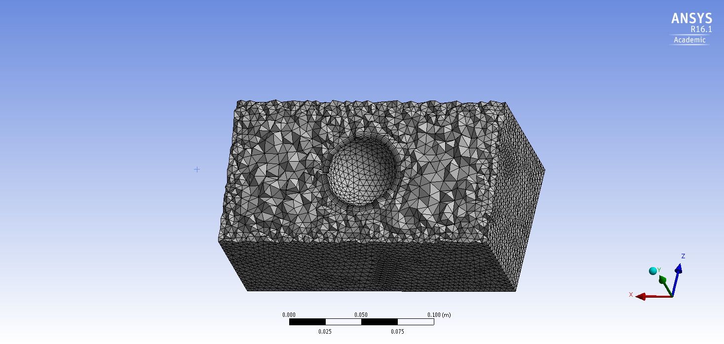
Meshing is the task of dividing the geometry into many small "elements".  
<!-- So there is a job of taking chunks of space and chopping them up into small control volumes. This process is called meshing, and each small piece is called either a "cell" or an "element". When I was learning CFD I used a bit of software called "Gambit", which was an absolute pig to learn but gave you a sense of superiority. Students hated learning the software because it was so impenetrable. Meshing was one of the most time-consuming parts of the process.

The quality of the mesh is really important and can have a dramatic impact on the quality of the results produced when you solve the equations. There are rules and heuristics about what makes a good mesh. You knew in your head how to get to a good mesh, but it was a time-consuming process. You could spend a long time painstakingly crafting each cell manually, or let automatic meshing algorithms help speed the process up. But they weren't great.

Over the years, attempts have been made to modernise the process. In the current state of the art, two things are true. Firstly, automatic meshing algorithms are actually very good. You can now just tell the software. Secondly, as computer resources have become cheaper, you can be a little more relaxed about using extra elements unwisely.

-->

![A rectangular block of fluid meshed with irregular grey triangular and tetrahedral cells, cut away to show a sphere inside it. The cells are small and tightly packed around the sphere, with thin layers wrapped around its surface, and larger further away.](https://mee-labsheets.shef.ac.uk/api/files/pbc_1321337024/f3ubh95a2n3ev2q/figure1_je7q3r944p.png)
: A tetrahedral mesh around a sphere, with inflation layers at its surface.

* The quality of the mesh has a dramatic impact on the results produced by the simulation. 
* Meshing is becoming an increasingly automated process.

## Pre-processing

The mesh divides the fluid into cells. We now set up the calculation:

* **Which physics?** Turbulence, heat transfer, chemical reactions.
* **Which fluid?** Air, water, and its material properties.
* **What happens at the boundaries?** Flow entering, flow leaving, solid walls.
* **How should the calculation run?** Solution methods and solver settings.

Each of these decisions will have an impact on the result of the simulation. 


The same mesh can be used for different calculations by changing these choices.


## Solved by numerical methods

* Some equations can be solved analytically. 
* Any question where the function of the unknown variable produces a known result can be solved _numerically_.
* For example
$$x = \cos x$$
$$\cos x-x = 0$$


* Use a "predictor-corrector" method.
$$r_n = \cos x_n - x_n$$

* where $r_n$ is the _residual_. 

##  Predictor-corrector

Start between $0$ and $1$; keep the half with a sign change. Angles are in radians.

| Guess | Calculation | Residual | New guess |
|------:|:------------|---------:|----------:|
| $0.5$ | $\cos(0.5) - 0.5 =$ | $+0.3776$ | $0.75$ |
| $0.75$ | $\cos(0.75) - 0.75 =$ | $-0.0183$ | $0.625$ |
| $0.625$ | $\cos(0.625) - 0.625 =$ | $+0.1860$ | $0.6875$ |
| $0.6875$ | $\cos(0.6875) - 0.6875 =$ | $+0.0853$ | $0.71875$ |
| $0.71875$ | $\cos(0.71875) - 0.71875 =$ | $+0.0339$ | $0.734375$ |
| $0.734375$ | $\cos(0.734375) - 0.734375 =$ | $+0.0079$ | $0.742188$ |
| $0.742188$ | $\cos(0.742188) - 0.742188 =$ | $-0.0052$ | $0.738281$ |
| $0.738281$ | $\cos(0.738281) - 0.738281 =$ | $+0.0013$ | $0.740234$ |

<!-- Bisection retains two endpoints with residuals of opposite signs. Initially r(0) = 1 and r(1) = cos(1) - 1, approximately -0.4597. Each guess is the midpoint. If its residual is positive, replace the lower endpoint; if negative, replace the upper endpoint. The new guess is the midpoint of the retained interval, not necessarily the average of the last two guesses.

The retained intervals after the eight rows are [0.5, 1], [0.5, 0.75], [0.625, 0.75], [0.6875, 0.75], [0.71875, 0.75], [0.734375, 0.75], [0.734375, 0.742188] and [0.738281, 0.742188]. Guesses and interval endpoints are displayed to at most six decimal places, and residuals to four; the calculation uses unrounded values internally. The interval halves each time, but the residual magnitude need not decrease on every row (compare 0.75 and 0.625). Continuing approaches x = 0.739085...; a stopping criterion may use a small absolute residual or a sufficiently narrow interval. -->

* For most practical flows, the Navier–Stokes equations have no known analytical solution, so we solve them approximately using numerical methods.

##  Residuals

![A logarithmic CFD residual plot with seven distinctly coloured curves falling over successive iterations and levelling off at separated magnitudes. Each curve is labelled beside its endpoint. Continuity stays highest and energy falls lowest.](/diagrams/cfd-residuals-convergence.svg)
: Residuals fall as the solver iterates, then level off at different magnitudes.

<!-- Schematic residual histories inspired by the supplied Fluent screenshot, not measured simulation data. The equal vertical steps are orders of magnitude on a logarithmic scale. Residuals can fluctuate and plateau; small residuals indicate that the discretised equations are being satisfied, but do not by themselves establish mesh independence or agreement with experiment. -->

## Post-processing

<!-- * CFD generates a vast quantity of numbers - proportional to the number of elements.
* Post process is a way to transform this into something useful. 
-->
. . . 

What you _think_ a valuable result from CFD is

![Coloured streamlines sweeping past a sphere whose surface is shaded from blue on one side to red on the other.](/images/cfd_streamline_sphere.jpg)
: Pictures: streamlines and surface colouring for flow past a sphere.

What an _actually valuable_ result from CFD is

![Ansys Fluent's force report for the sphere, with the total force of -0.148 N circled in red.](/images/cfd_drag_output.jpg)
: Numbers: Fluent's force report, with the total drag on the sphere circled.


## Validation

Validation checks whether the simulation gives the _right_ answer.

**But what does “right” mean?**

::: {.fragment}
::: {.keypoint}
The answer predicts what would happen if the simulated conditions existed in the real world. 
::: 

* Simulations consist of assumptions, estimations, decisions (Mesh, models, physics and numerics) which all influence the answer.
* The simulation will **merrily** and **convincingly** generate you _an_ answer. 
* Just like analytical calculations, web searches, AI output, you need to check what is being produced is correct. 
::: {.keypoint}
A convincing answer still needs validation.
:::

:::


## You are liable.


> THE ENTIRE RISK ARISING OUT OF THEIR USE REMAINS WITH THE RECIPIENT. IN NO EVENT SHALL ANSYS AND/OR ITS RESPECTIVE SUPPLIERS BE LIABLE FOR ANY DIRECT, CONSEQUENTIAL, INCIDENTAL, SPECIAL, PUNITIVE OR OTHER DAMAGES WHATSOEVER (INCLUDING WITHOUT LIMITATION, DAMAGES FOR LOSS OF BUSINESS PROFITS, BUSINESS INTERRUPTION, OR LOSS OF BUSINESS INFORMATION), EVEN IF ANSYS HAS BEEN ADVISED OF THE POSSIBILITY OF SUCH DAMAGES.

https://ansys.synopsys.com/legal/legal-notices

## How to validate CFD results.
Compare the simulation result to
* Experimental results (not necessarily yours)
* Theoretical result (that has been validated)
* Another CFD result (that has been validated)

If the result of the simulation is already known to validate against, why do the CFD simulation in the first place?


<!-- Pause after asking what "correct" means. First click: agreement with what would happen in the real world, to the accuracy needed for the intended use. Second click: modelling choices, assumptions and the need for independent evidence. Third click: the question of why CFD is useful if validation requires a known answer.

Validation establishes confidence through comparison with physical evidence rather than proving an exact answer. Mesh independence and numerical convergence help check the numerical solution; physical validation checks how well the model represents reality. A method can be validated against known cases and then used to investigate new cases within its demonstrated range of applicability. The final question is left open for discussion. -->

## Summary

* CFD complements theory and experiment; all three inform each other.
* Computing advances have made CFD more accessible for numerical experiments.
* Start with an engineering question and plan the study before simulating.
* The steps in the workflow for a CFD simulation:
    * **Geometry creation:** define the fluid domain.
    * **Meshing:** divide it into cells; mesh quality affects the results.
    * **Pre-processing:** choose physics, fluid properties, boundaries and solver settings.
    * **Solving:** solve conservation equations numerically and monitor residuals.
    * **Post-processing:** extract useful engineering quantities, such as drag.
    * **Validation:** check against real-world evidence before trusting a convincing answer.


<!-- 
Not included in this talk, but maybe will put in later 

Good for some tasks, not for others; it takes some wisdom to know when and where to use it. This is what humans are good at and AI is less good at. AI will make the button clicking easier, but to a certain extent it is the practice and button clicking that build the holistic understanding. This also brings us on to computation and symmetry: use tricks like 2D and modelling only half the flow when needed.
-->
