MEC Lecture · Computational Fluid Dynamics University of Sheffield

Pretty Convincing?

My Opinionated Introduction to CFD

Presenter Professor Andrew Garrard MEng(hons) PhD CEng FIMechE PFHEA

Details MAC118
8 August 2026

What we will learn today

By the end of this lecture you will be able to:

Outline how CFD developed into its current state of the art
Explain why and how CFD is used alongside experiment and theory
Describe the steps involved in simulating a fluid flow numerically
Relate broad CFD concepts to the applications in the tutorials

Introduction

CFD stands for

C - Computational
F - Fluid
D - Dynamics

Computational fluid dynamics (CFD) is a branch of both fluid mechanics and computational physics that uses numerical analysis and data structures to analyze and solve problems that involve flows.

Wikipedia, "Computational fluid dynamics"

Alternatively

Colours for Directors

a.k.a

"The Beautiful Lie"

Contemporary uses of CFD

A simulation to determine safety for Urban Air Mobility.

A single two-bladed rotor hovering above a grey ground plane, surrounded by a dense tangle of thin blue vortex tubes that spread out across the ground, with brighter green and magenta rings trailing just below the rotor tips. — Hovering quadcopter rotor in ground effect. Image: Patricia Ventura Diaz and D-G Caprace, Tim Sandstrom. NASA/Ames.

Watch the simulations on the NASA page

A history of CFD

Fluid mechanics before computers

From the 17th to the 19th century, fluid mechanics was split into two disciplines.

Early CFD

CFD arrives, and it is not well defined as either theory or experiment.

A third way

Three fields of fluid mechanics, of equal importance, each informing the others.

Driving and bottlenecking CFD progress

Commercial computers

Pushing boundaries in fluid mechanics

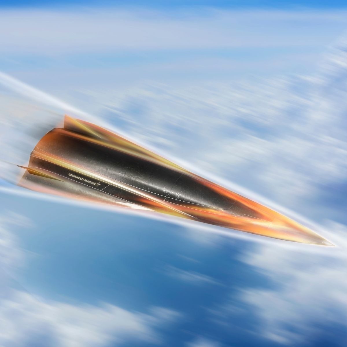
A slender dart-shaped vehicle streaking through high cloud, its leading edges glowing orange with the heat of the airflow. — A Lockheed Martin hypersonic vehicle.

Pushing boundaries in fluid mechanics

A flow visualization of NASA’s X‑59 supersonic, low-boom aircraft concept. This computational fluid dynamics simulation, produced on the Pleiades supercomputer using the NAS-developed Launch Ascent and Vehicle Aerodynamics (LAVA) code, will be used to help determine which components contribute to the pressure signatures below the aircraft that create the sonic boom in flight. Red and blue represent high and low pressure, respectively; the symmetry plane—which bisects the vehicle along its center line—is colored by Mach number. James Jensen, NASA/Ames.

https://nas.nasa.gov/pubs/stories/2021/feature_X-59.html

Wind tunnels

The most powerful wind tunnel in the world.

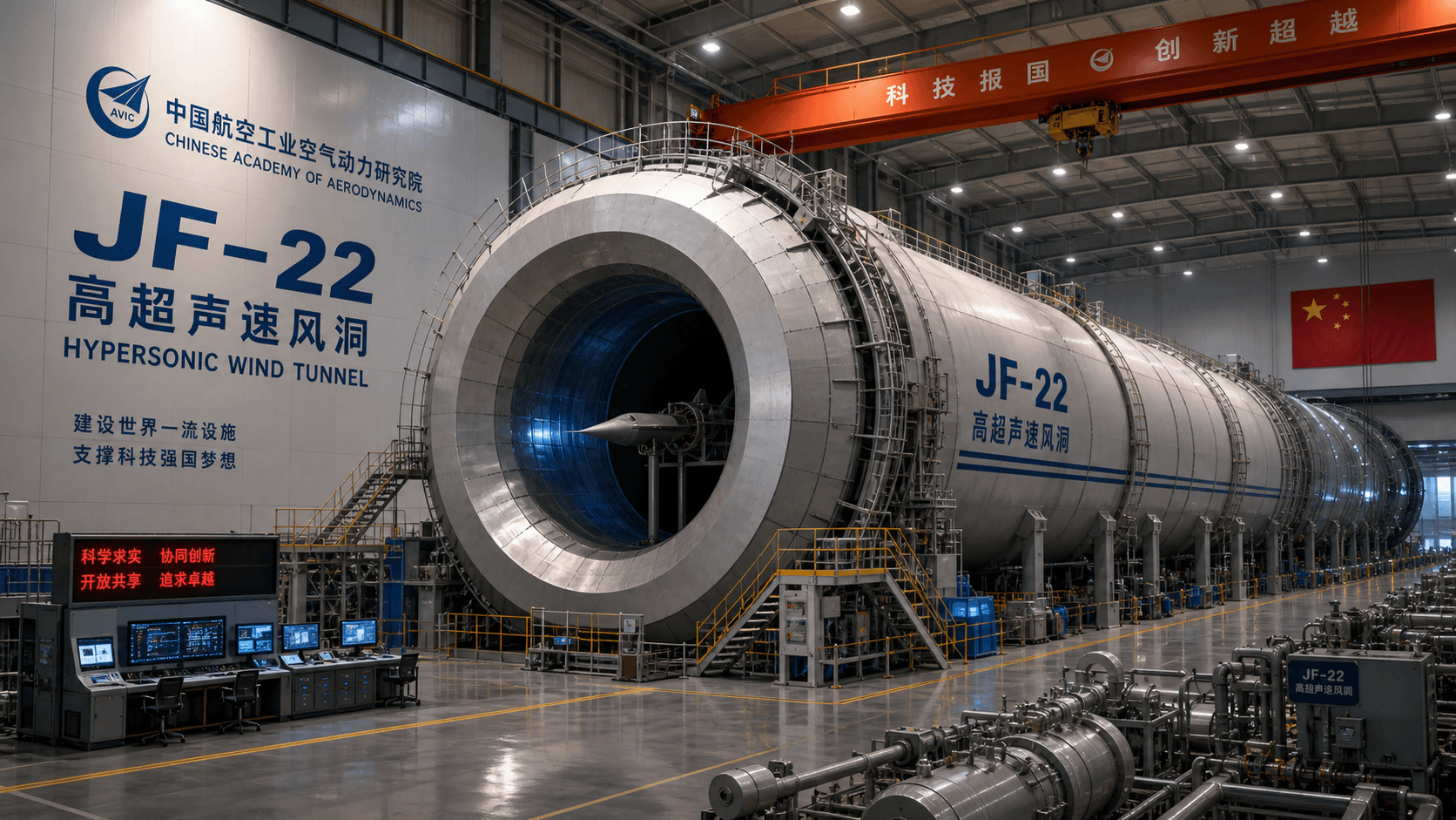
The JF-22 hypersonic wind tunnel at the Chinese Academy of Aerodynamics. Pandaily, https://pandaily.com/jf22-hypersonic-wind-tunnel-10km-jul2026, obtained 2026-09-11.

A couple of issues with wind tunnels

Power

The JF-22 uses 15 GW of power.

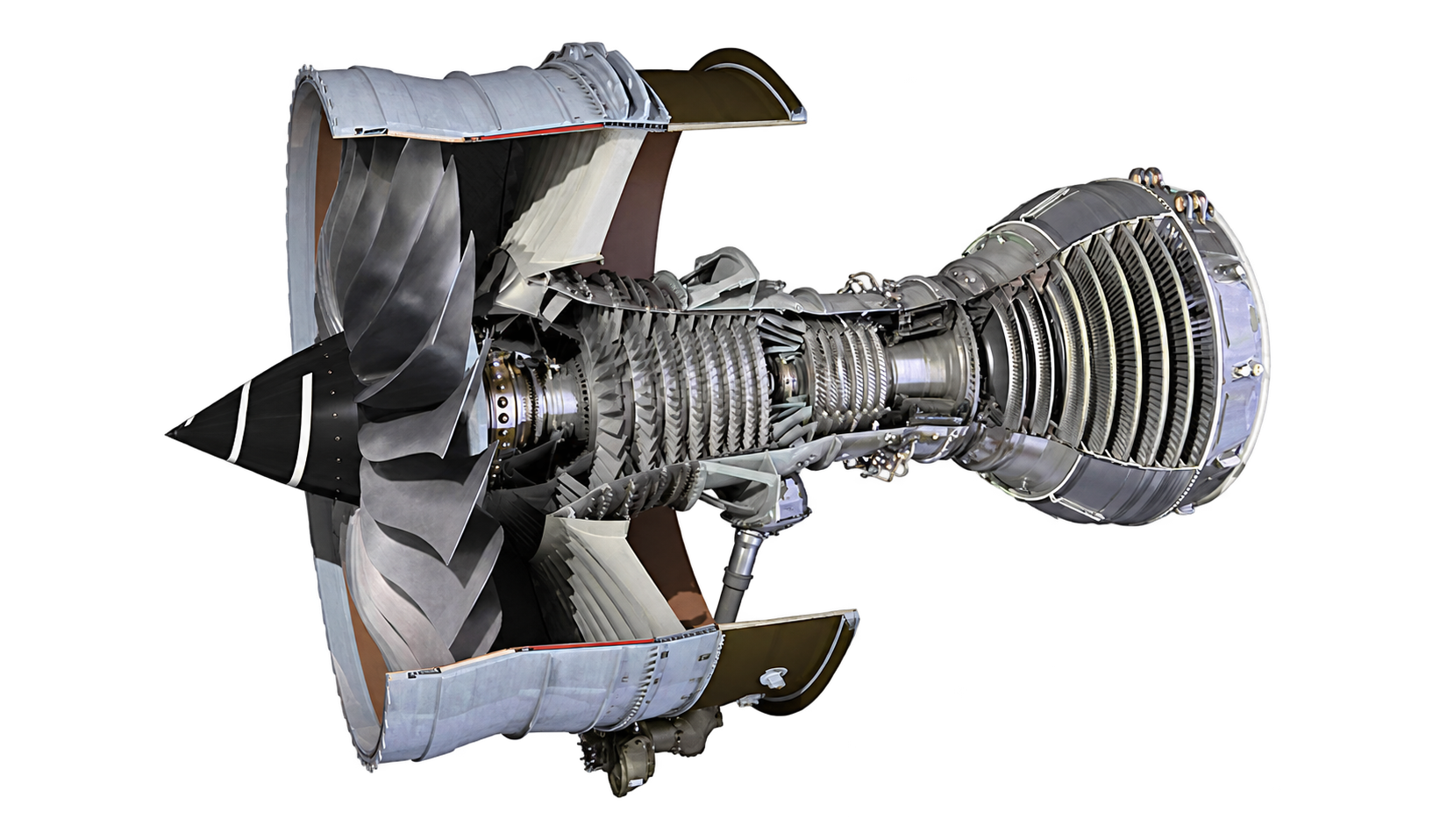
A Rolls-Royce Trent XWB turbofan, cut away along its length. — 180 × Trent XWB engines.

Iron Man in flight in his red and gold armour. — 5 × Iron Men.

Scale

The JF-22 has a working section of 4 m.

Real planes are bigger than 4 m across.

$$Re = \frac{\rho V L}{\mu}$$

The run time is less than 120 ms.

Why use CFD?

Cheaper
Safer
Unphysical problems
Complete dataset
Data after experiment
Increasingly automated

But...

No exact solution
No idea if the answer is correct – "black box engineering"
Good for some situations, not for others - this requires some wisdom

Why I like CFD

I can work independently
Easy "what if" scenarios
Work from anywhere

Numerical experiment

CFD can be a portable, cheap wind tunnel.

Numerical experiment

Used to test a model, theory or hypothesis.
Fewer factors are outside your control than in a physical experiment, but not none.
Error will occur and has to be understood and accounted for.
Good experimental design needs to be performed before starting.
Experiments should adhere to the scientific method.
Focus should always be maintained on the reasons for conducting the experiment.

Something for everyone

The CFD stack: every answer rests on six layers the engineer never sees.

Some of my work

Simulation of a "personal cloud"
Prediction of smoke ingress and movement in offshore installations
GRP spraying of boat hulls
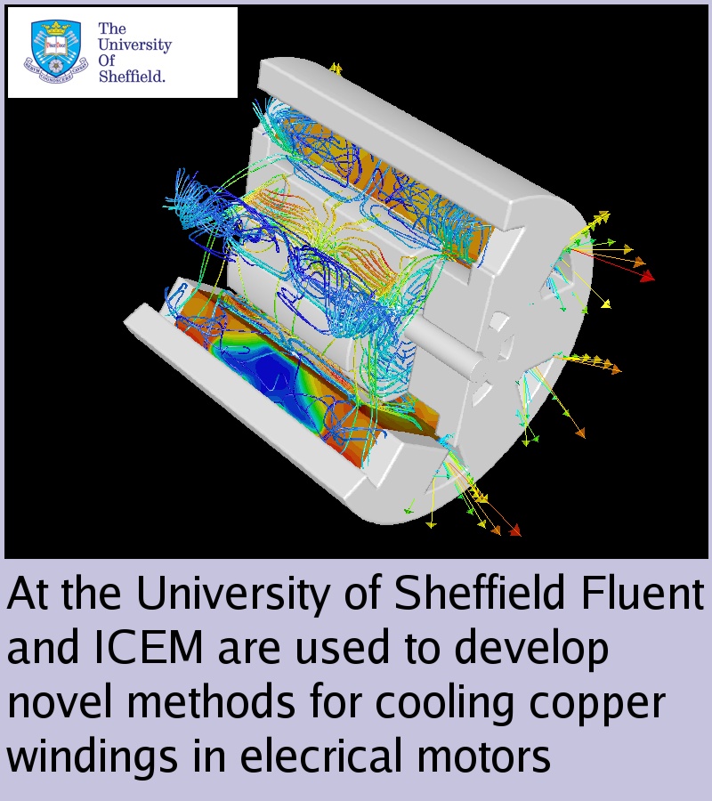
Electric motor cooling
Fuel cell electrochemical modelling

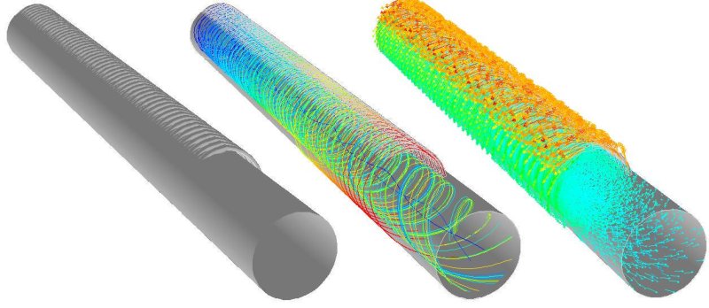
Cutaway of a motor with coloured streamlines through the windings and velocity vectors fanning past the rotor poles. — Cooling and windage loss in a switched reluctance motor.

Three stages side by side: a bare cylindrical manifold, streamlines spiralling along it, then a dense vector field. — Swirl in a fuel cell stack manifold.

Commercial software

In the recent past

Dedicated CFD platforms

Fluent
CFX
STAR-CD
COMSOL (general)
OpenFOAM (open source)

Now

Large multiphysics packages

Ansys (Synopsys)
Dassault Systèmes
CAD bolt-ons (not very good)
COMSOL (general)
OpenFOAM (open source)

At Sheffield we use Ansys Fluent.

In 1979, Jim Swithenbank, at the time Professor of Chemical Engineering at the University of Sheffield, invited Boysan back to Sheffield to help him develop a code capable of interactively defining geometry and boundary conditions for a specific problem involving cyclone separators. The resulting software was developed with a student, Bill Ayers, as part of his final year research project and was published in the Transactions of the Institute of Chemical Engineers. With the permission of the authors, the editor of the publication added a note that readers could contact the authors to obtain a copy of the source code. Swithenbank and Boysan were surprised to receive several hundred requests for the code, alerting them to the commercial potential of an interactive CFD code. https://www.nafems.org/blog/posts/analysis-origins-fluent/?srsltid=AfmBOopakyIaFfFPIGLA3VZjCl19QUbzOLI8D3czKXd6mK8pdP1zOttu

Fluent started in Sheffield

A crowded, brightly coloured painting of Sheffield: Victorian buildings, a pub, a tram, a football match in the foreground, and the white Fluent offices flying international flags at the back. — Joe Scarborough's painting of Fluent Europe's Sheffield, commissioned in 2000.

How CFD works

From equations to numbers.

The Navier–Stokes equations

Conservation of mass

$$\frac{\partial u}{\partial x} + \frac{\partial v}{\partial y} + \frac{\partial w}{\partial z} = 0$$

Conservation of momentum, in $x$, $y$ and $z$

$$\rho\left(\frac{\partial u}{\partial t} + u\frac{\partial u}{\partial x} + v\frac{\partial u}{\partial y} + w\frac{\partial u}{\partial z}\right) = -\frac{\partial p}{\partial x} + \mu\left(\frac{\partial^{2} u}{\partial x^{2}} + \frac{\partial^{2} u}{\partial y^{2}} + \frac{\partial^{2} u}{\partial z^{2}}\right) + \rho g_{x}$$

$$\rho\left(\frac{\partial v}{\partial t} + u\frac{\partial v}{\partial x} + v\frac{\partial v}{\partial y} + w\frac{\partial v}{\partial z}\right) = -\frac{\partial p}{\partial y} + \mu\left(\frac{\partial^{2} v}{\partial x^{2}} + \frac{\partial^{2} v}{\partial y^{2}} + \frac{\partial^{2} v}{\partial z^{2}}\right) + \rho g_{y}$$

$$\rho\left(\frac{\partial w}{\partial t} + u\frac{\partial w}{\partial x} + v\frac{\partial w}{\partial y} + w\frac{\partial w}{\partial z}\right) = -\frac{\partial p}{\partial z} + \mu\left(\frac{\partial^{2} w}{\partial x^{2}} + \frac{\partial^{2} w}{\partial y^{2}} + \frac{\partial^{2} w}{\partial z^{2}}\right) + \rho g_{z}$$

$u$, $v$, $w$ velocity components · $p$ pressure · $\rho$ density · $\mu$ dynamic viscosity

Solving the Navier–Stokes equations

The Navier–Stokes equations cannot be solved analytically.

Despite what Sam Altman says

Screen grab of BBC News from 8 September 2026, showing Sam Altman's face as the cover image and the headline "OpenAI says it cracked 90-year-old maths problem in 88 hours". https://www.bbc.co.uk/news/articles/cy7zygy3rl2o, 8 September 2026. — OpenAI didn't solve the Navier–Stokes equations. From BBC News, https://www.bbc.co.uk/news/articles/cy7zygy3rl2o, 8 September 2026.

Basic conservation equation

Mass is conserved. The mass entering across the boundary minus the mass leaving across it is the mass accumulated inside.

Momentum is also conserved in the same way, but has a third route in: forces on the boundary.

Discretising

Typical CFD simulation workflow

The steps of running a CFD simulation.

The more holistic CFD simulation workflow

Running the simulation is one step of six in a CFD study.

The complete CFD simulation workflow

The whole simulation pipeline is one box in the study.

Geometry creation

This is basically CAD. But the fluid needs to be created, not (necessarily) the solid.

To predict drag, mesh the air surrounding the rocket. The rocket’s surface forms a boundary of the fluid domain.

Meshing

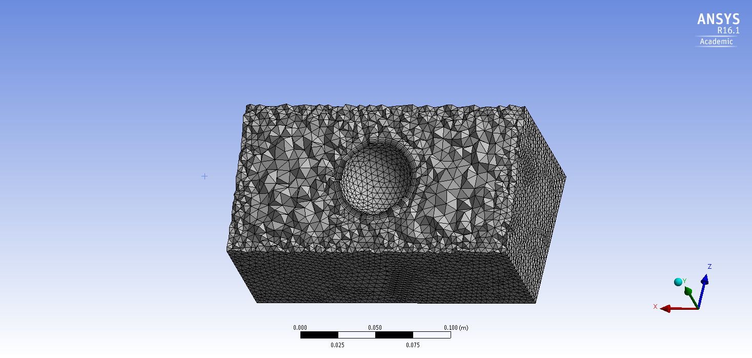
Meshing is the task of dividing the geometry into many small "elements".

A rectangular block of fluid meshed with irregular grey triangular and tetrahedral cells, cut away to show a sphere inside it. The cells are small and tightly packed around the sphere, with thin layers wrapped around its surface, and larger further away. — A tetrahedral mesh around a sphere, with inflation layers at its surface.

The quality of the mesh has a dramatic impact on the results produced by the simulation.
Meshing is becoming an increasingly automated process.

So there is a job of taking chunks of space and chopping them up into small control volumes. This process is called meshing, and each small piece is called either a "cell" or an "element". When I was learning CFD I used a bit of software called "Gambit", which was an absolute pig to learn but gave you a sense of superiority. Students hated learning the software because it was so impenetrable. Meshing was one of the most time-consuming parts of the process.

The quality of the mesh is really important and can have a dramatic impact on the quality of the results produced when you solve the equations. There are rules and heuristics about what makes a good mesh. You knew in your head how to get to a good mesh, but it was a time-consuming process. You could spend a long time painstakingly crafting each cell manually, or let automatic meshing algorithms help speed the process up. But they weren't great.

Over the years, attempts have been made to modernise the process. In the current state of the art, two things are true. Firstly, automatic meshing algorithms are actually very good. You can now just tell the software. Secondly, as computer resources have become cheaper, you can be a little more relaxed about using extra elements unwisely.

Pre-processing

The mesh divides the fluid into cells. We now set up the calculation:

Which physics? Turbulence, heat transfer, chemical reactions.
Which fluid? Air, water, and its material properties.
What happens at the boundaries? Flow entering, flow leaving, solid walls.
How should the calculation run? Solution methods and solver settings.

Each of these decisions will have an impact on the result of the simulation.

The same mesh can be used for different calculations by changing these choices.

Solved by numerical methods

Some equations can be solved analytically.
Any question where the function of the unknown variable produces a known result can be solved numerically.
For example $$x = \cos x$$ $$\cos x-x = 0$$
Use a "predictor-corrector" method. $$r_n = \cos x_n - x_n$$
where $r_n$ is the residual.

Predictor-corrector

Start between $0$ and $1$; keep the half with a sign change. Angles are in radians.

Guess	Calculation	Residual	New guess
$0.5$	$\cos(0.5) - 0.5 =$	$+0.3776$	$0.75$
$0.75$	$\cos(0.75) - 0.75 =$	$-0.0183$	$0.625$
$0.625$	$\cos(0.625) - 0.625 =$	$+0.1860$	$0.6875$
$0.6875$	$\cos(0.6875) - 0.6875 =$	$+0.0853$	$0.71875$
$0.71875$	$\cos(0.71875) - 0.71875 =$	$+0.0339$	$0.734375$
$0.734375$	$\cos(0.734375) - 0.734375 =$	$+0.0079$	$0.742188$
$0.742188$	$\cos(0.742188) - 0.742188 =$	$-0.0052$	$0.738281$
$0.738281$	$\cos(0.738281) - 0.738281 =$	$+0.0013$	$0.740234$

For most practical flows, the Navier–Stokes equations have no known analytical solution, so we solve them approximately using numerical methods.

Bisection retains two endpoints with residuals of opposite signs. Initially r(0) = 1 and r(1) = cos(1) - 1, approximately -0.4597. Each guess is the midpoint. If its residual is positive, replace the lower endpoint; if negative, replace the upper endpoint. The new guess is the midpoint of the retained interval, not necessarily the average of the last two guesses.

The retained intervals after the eight rows are [0.5, 1], [0.5, 0.75], [0.625, 0.75], [0.6875, 0.75], [0.71875, 0.75], [0.734375, 0.75], [0.734375, 0.742188] and [0.738281, 0.742188]. Guesses and interval endpoints are displayed to at most six decimal places, and residuals to four; the calculation uses unrounded values internally. The interval halves each time, but the residual magnitude need not decrease on every row (compare 0.75 and 0.625). Continuing approaches x = 0.739085...; a stopping criterion may use a small absolute residual or a sufficiently narrow interval.

Residuals

Residuals fall as the solver iterates, then level off at different magnitudes.

Post-processing

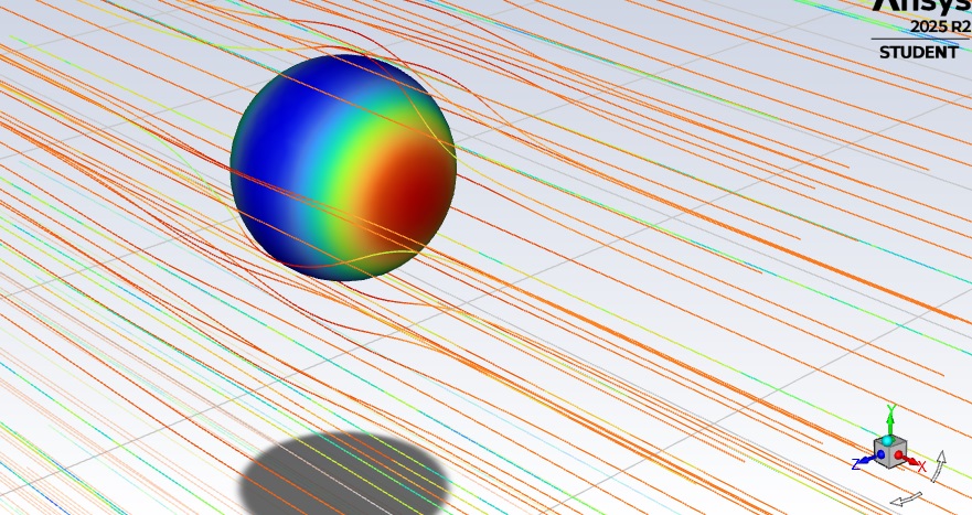
What you think a valuable result from CFD is

Coloured streamlines sweeping past a sphere whose surface is shaded from blue on one side to red on the other. — Pictures: streamlines and surface colouring for flow past a sphere.

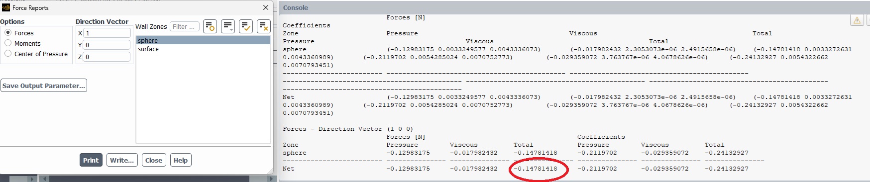
What an actually valuable result from CFD is

Ansys Fluent's force report for the sphere, with the total force of -0.148 N circled in red. — Numbers: Fluent's force report, with the total drag on the sphere circled.

Validation

Validation checks whether the simulation gives the right answer.

But what does “right” mean?

The answer predicts what would happen if the simulated conditions existed in the real world.

Simulations consist of assumptions, estimations, decisions (Mesh, models, physics and numerics) which all influence the answer.
The simulation will merrily and convincingly generate you an answer.
Just like analytical calculations, web searches, AI output, you need to check what is being produced is correct.

A convincing answer still needs validation.

You are liable.

THE ENTIRE RISK ARISING OUT OF THEIR USE REMAINS WITH THE RECIPIENT. IN NO EVENT SHALL ANSYS AND/OR ITS RESPECTIVE SUPPLIERS BE LIABLE FOR ANY DIRECT, CONSEQUENTIAL, INCIDENTAL, SPECIAL, PUNITIVE OR OTHER DAMAGES WHATSOEVER (INCLUDING WITHOUT LIMITATION, DAMAGES FOR LOSS OF BUSINESS PROFITS, BUSINESS INTERRUPTION, OR LOSS OF BUSINESS INFORMATION), EVEN IF ANSYS HAS BEEN ADVISED OF THE POSSIBILITY OF SUCH DAMAGES.

https://ansys.synopsys.com/legal/legal-notices

How to validate CFD results.

Compare the simulation result to

Experimental results (not necessarily yours)
Theoretical result (that has been validated)
Another CFD result (that has been validated)

If the result of the simulation is already known to validate against, why do the CFD simulation in the first place?

Summary

CFD complements theory and experiment; all three inform each other.
Computing advances have made CFD more accessible for numerical experiments.
Start with an engineering question and plan the study before simulating.
The steps in the workflow for a CFD simulation:
- Geometry creation: define the fluid domain.
- Meshing: divide it into cells; mesh quality affects the results.
- Pre-processing: choose physics, fluid properties, boundaries and solver settings.
- Solving: solve conservation equations numerically and monitor residuals.
- Post-processing: extract useful engineering quantities, such as drag.
- Validation: check against real-world evidence before trusting a convincing answer.