Before starting this tutorial:
Step 1: Open the project file used to find the drag on the sphere in Workbench. Open the Fluent software to reach the endpoint of the last tutorial.
In the remaining steps, we will add a thermal model to the previously created model that only simulated the aerodynamic drag on the sphere. There are only three steps in this process.
Step 2: Enable the energy equation. From the Models menu of the tree outline (where you previously set the turbulence model), double-click Energy and ensure it is selected.
When you turn on the energy module, you are instructing the software to solve for an additional conservation equation (in this case, the conservation of energy) and set up a new solution variable in every cell to capture the results of this conservation equation. The new solution variable is "temperature," so along with X-velocity, Y-velocity, etc., each cell will also hold a temperature value with the energy equation enabled. With this model enabled, new options become available in other parts of the simulation setup.
Step 3: Changing material properties. In isothermal simulations, material properties (such as density) have been set at constant values. However, with the energy equation enabled and temperature data available in all cells, these values can be set as functions of temperature. To do this, go to the Materials panel of the tree outline and double-click on the fluid material. Different models to calculate material properties (rather than specifying them as constant values) can be selected from the drop-down menus. For example, density can be calculated from the known pressure and temperature using the ideal gas equation.
Step 4: Set thermal boundary conditions. With the energy equation enabled and a conservation of energy equation solving for temperature, boundary conditions for this equation need to be specified. When opening the boundary condition panels with the energy equation enabled, the Thermal tabs become available. Open all the previously set boundary conditions and input thermal boundary conditions. Pay special attention to the boundary condition representing the sphere inside the domain. The thermal tab of the boundary conditions panel allows a heat flux or a temperature to be applied. Calculate the heat flux (in Watts per meter squared) out of the sphere and input this into the panel.
To extract the results of this change, you will need to reinitialize the simulation (if required) and rerun the calculation.
The mesh used for CFD simulation is created by dividing the computational domain into discrete pieces of space. On a surface, the two-dimensional shapes that divide the space are called facets. Facets are small portions of the larger surface, and the vertices (plural of vertex) are the points between them.
Consider, for example, the surface shown on the left in the image below, with the facets shown in blue and the vertices shown in red.
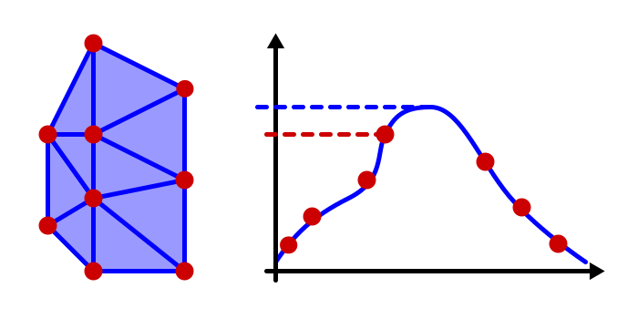
When calculations are performed, the CFD numerics will store "facet" values, which are the point values of temperature at the center of the elements. It can produce the values at the vertices by interpolating between cell center (facet) values.
To the right of the figure, you can see the same surface with the facet values of a solution variable (for example, temperature) plotted in blue and the vertex values plotted as points in red. The highest facet value is larger than the highest vertex value.
In the real world, there is a continuous distribution of properties such as temperature across a surface. In a simulation, where the space is divided into discrete pieces, the values of these properties are calculated at the vertices and the facets. When you ask the computer to display the output, you can choose either vertex or facet values.