In this tutorial, we will use the Ansys Fluent software to open a "workbench" file that contains a 2D, axisymmetric geometry and mesh of a bellmouth inlet. This bellmouth inlet draws air from the surroundings into a 92 mm diameter pipe. Inside the Fluent software, we will perform the pre-processing necessary to set up a CFD simulation. We will enable an axisymmetric model, instruct the software to model turbulence, check the material properties for air, and set all the boundary conditions. We will then initialize and run the simulation. Once the calculation is completed, we will post-process the results by creating contours of pressure and velocity. We will produce a graph of the velocity profile, which will allow us to determine the boundary layer thickness and compare the result with empirical predictions.
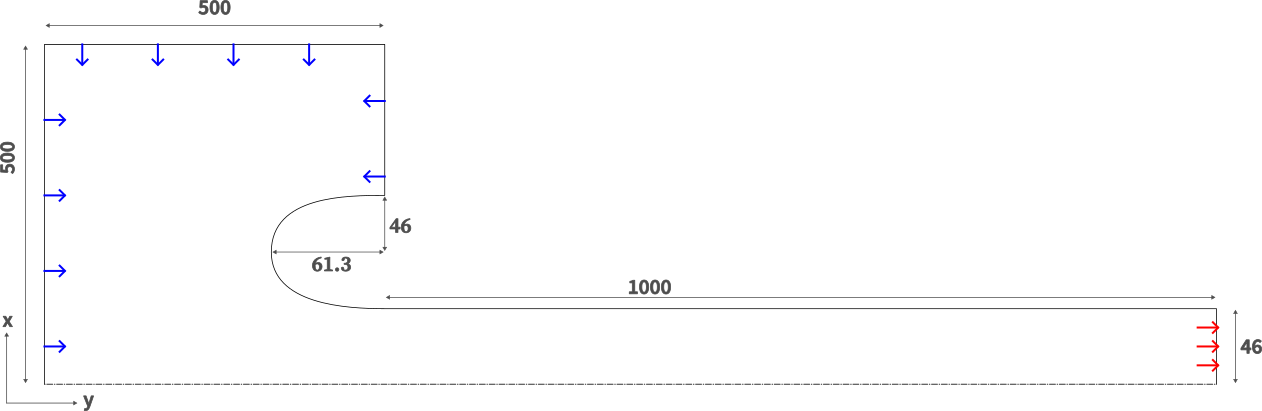
A schematic of half the bellmouth inlet is shown above. The distances are shown in millimeters. Only half of the domain is created and meshed, as it is going to be modeled as axisymmetric around the center line, shown as dot dashes. Not to scale.
Time to complete: 40 minutes.
Pre-requisite tutorials: Ansys Workbench Familiarisation
Software version: This tutorial was prepared using Ansys 2024 R1. There may be minor differences when following the tutorial in later versions.
Before starting this tutorial:
Step 1: Open the project file. From the Workbench interface, open the downloaded project file by selecting File and then Open from the top menu. Navigate to where the project file is, select it, and click Open. The Project Schematic should now display the Fluid Flow (Fluent) system A.
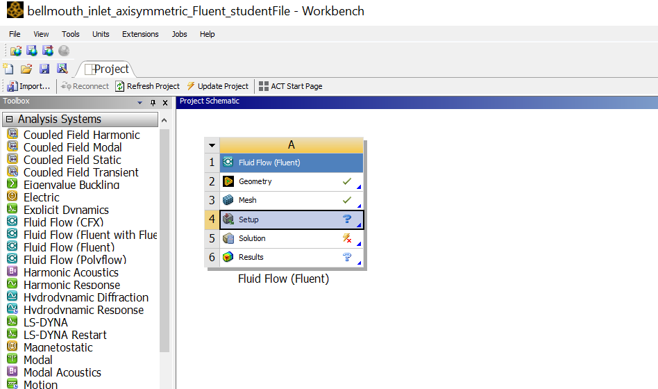
Step 1b: Update the project if needed. If a lightning strike appears in the Mesh or Setup lines of the system, this implies that the connection between the Mesh system and the Fluent system needs updating. This can be done using the Update Project button on the top menu. In the example above, with the green tick in the Mesh row and a question mark in the Setup row, you do not need to update the project. If you do update, you may need to wait a while for this to process, and it may end with an error message stating, "Update failed for the Solution component in Fluent. Update solution Failed." Do not worry about this – it is attempting to populate the project files with results from a CFD calculation that has not been conducted yet. Just press OK. If the firewall dialogue box appears, this can usually be dismissed with the "Cancel" option, without causing any problems. You may need to do this several times.
Step 2: Open Fluent Software. Double-click Setup on the 4th row of the Fluid Flow (Fluent) system A on the project schematic. This will open the Fluent Launcher window. Click Setup or Start to open the Fluent software. This may take a moment to read in the data and display the interface. Dismiss any update messages displayed in the Fluent window by clicking OK.
In the Fluent Launcher window, we were presented with a few options. One was to select either a 2D or 3D simulation. In this case, the mesh has been connected to the Fluent system in the Workbench, so it knows the incoming mesh is 2D and this option is selected and the ability to change it is greyed out. There is also an option to select the number of processes across which the simulations should be parallelized. For large meshes, it can be faster to distribute the calculation across multiple processes if you have them in your computer. In this case, our mesh is small, so we will accept whatever has been chosen by default.
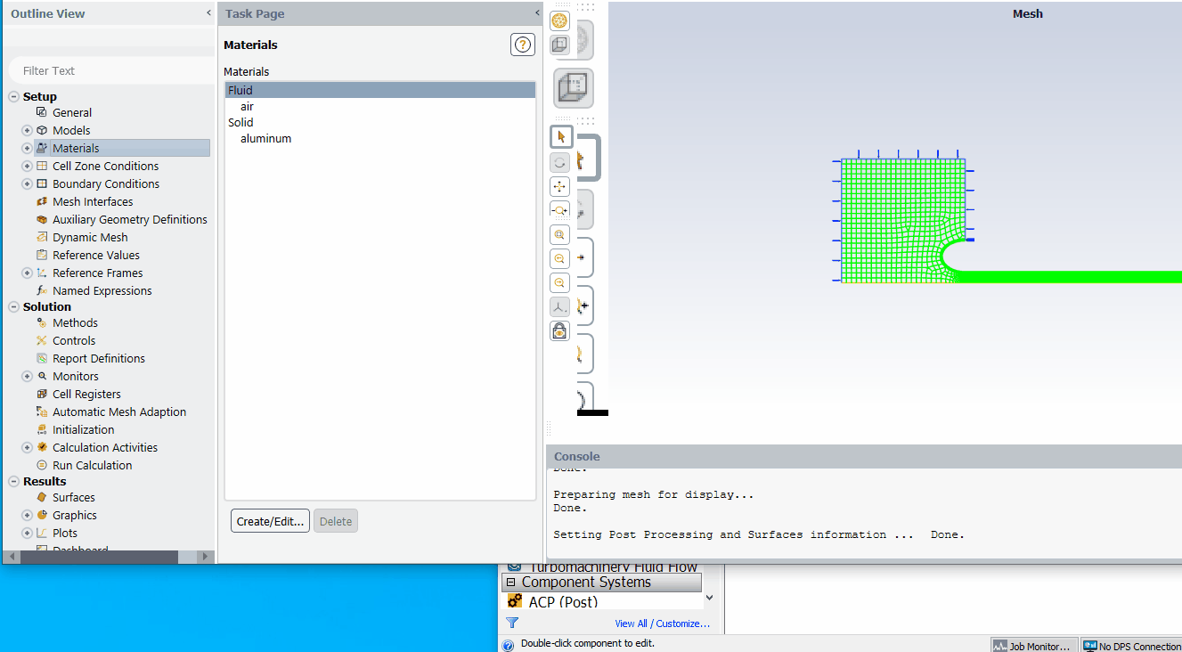
Step 3: Check the mesh. Double click General in the Outline View to open the General options in the Task Page. It is sensible to run a check on all incoming meshes to see if any errors are detected. Under the Mesh options of the Task Page, click Check. A series of data about the mesh will appear in the Console, and if all the checks are passed, this will terminate with the word Done.
Step 4: Apply axisymmetric model. Still within the General Task Page, under the Solver and 2D space options, select Axisymmetric.
The Axisymmetric model will calculate the simulation on the 2D mesh assuming that it represents a slice of a 3D object that would be created if the slice were rotated 360 degrees around the x-axis. The code has no option to specify the axis of rotation, it always uses the positive x-axis. Axisymmetric meshes must be built with this in mind.
Step 5: Apply a turbulence model. Expand the Models menu from the Outline View. Double click Viscous (SST k-omega) to open the Viscous Model options page. Under the Model options, ensure SST k-omega is selected. Click OK.
The "Viscous Model" page allows you to specify how turbulence is simulated. It is possible to run an inviscid simulation, with no friction, or a laminar simulation, where there is no turbulence. However, if your simulation requires turbulence (because the Reynolds number has exceeded the critical value), one of several different models needs to be chosen. In this case, we are going to use the k-omega model, which adds two more conservation equations and creates two variables in each cell to store values to account for the turbulence.
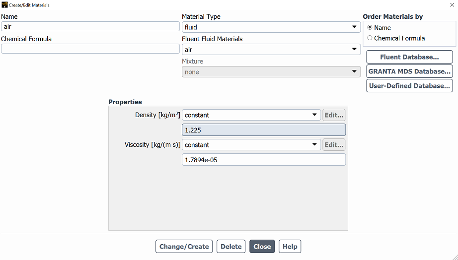
Step 6: Check material properties. Expand the Materials menu from the Outline View, and then expand the Fluid menu to reveal the default material, "air." Double-click air to bring up the properties of this material. Under the Properties menu, note the value of density and viscosity. Click Close. Close the material properties window.
In this part of the software, we can, if required, change the properties of air or create new materials. Our simulation is of air being drawn into a wind tunnel, so we can accept the default material and material properties. You can change the value of the material properties if you want.
In the next step, we will apply boundary conditions to any mesh elements at the edge of the domain. These are the boundary conditions the software needs to solve the governing equations. There needs to be a condition for every variable that is being solved for, in this case, x-velocity, y-velocity, pressure, and two variables to account for turbulence (k and omega), on every boundary surface. However, the Fluent software makes this process easier by allowing users to select physical boundary types, such as inlets, outlets, and walls, and determining how to set the appropriate variables for each equation. Fluent attempts to select the correct boundary condition type based on the name provided in the Mesher. If the boundary is called something like "pipe inlet," it may guess to apply a "velocity-inlet" boundary type. However, it can make decisions that might not have been your intention, so it is always good to check the boundary type that has been applied.
Step 6: Check boundary condition types. Double click Boundary Conditions in the Outline View and this will open the Boundary Conditions panel in the Task Page. Listed in the Task Page are previously named boundaries. Naming would typically happen during the meshing stage. In this case, these are Axis, Inlet, Outlet, and Wall. There may be some internal surfaces, but as these are not on the boundary of the domain, these do not need any conditions set for them. Single click axis in the boundary conditions list and note the entry in the "Type" dropdown at the bottom of the Task Page. Ensure that Type is set to "axis" and if not, select this from the dropdown. Work your way down the list to check the following types:
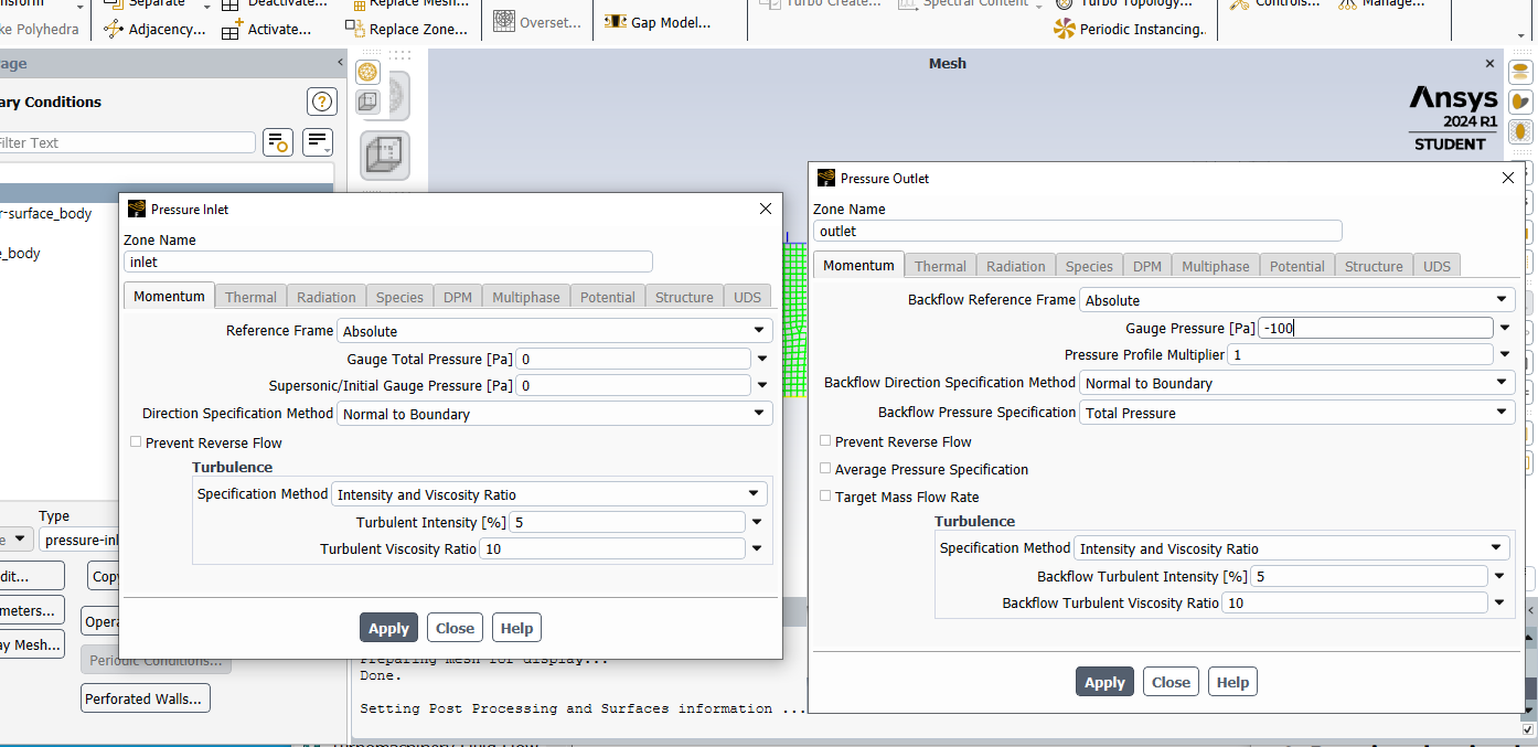
Step 7: Edit the inlet boundary conditions. Using the method above, change the inlet boundary to pressure-inlet. Double click inlet in the Task Page. This will bring up a window to allow you to edit the settings for the "pressure-inlet" type boundary conditions. The air into the wind tunnel will be drawn in from the atmosphere, which is at 0 Pa, gauge. Ensure the Gauge Pressure [Pa] in the inlet boundary condition panel is set to the default value of zero. Click Apply and then Close.
Step 8: Edit the outlet boundary conditions. Double click outlet in the Task Page. This will bring up a window to allow you to edit the settings for the "pressure-outlet" type boundary conditions. The air into the wind tunnel will be drawn in by the suction of a fan. Simulate this suction by setting the Gauge Pressure [Pa] to -100, using the method above. Click Apply and then Close.
In the next step we will initialize the calculation. As the calculation is an iterative, numerical method that updates the solutions based on a previous prediction, initial values are required. Values of every solution variable are required for every mesh element. Fortunately, there are tools built into the Fluent software to make this process easier.
Step 9: Initialization. Expand the Solution menu from the Tree Outline. Double click Initialization. In the Task Page, Under Solution Initialization, ensure Hybrid Initialization is selected. Click the Initialize button.
In Fluent, there are two common options for initialization, "Standard" or "Hybrid". In "Standard", you can specify values for each of the solution variables. The software will apply these values to all of the mesh elements. You can also call the values from each of the solution variable from any of the boundary conditions you have previously set up. In this case, because we don't know what the speed of the air inside the wind tunnel is going to be, we will allow the hybrid initiatlization to make an initial guess for us.
Step 10: Run the calculation. Within Solution in the Tree menu, double click Run Calculation. In the Task Page, under Parameters, enter 1000 in the Number of Iterations text entry box. Click Calculate. You should see the residuals appear in the Graphics window.
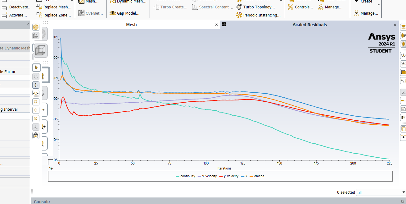
When selecting the number of iterations, in this case 1000, this is the maximum number of iterative calculations the software will perform. The software will stop calculating if the convergence criteria are reached before it has reached the maximum number of iterations. The default convergence criteria are set to all solutions variable reaching a residual value of 0.001. If you want to make the convergence criteria more strict, this can be set from the Monitors then Residuals option on the left hand menu. The values of Absolute Criteria could be reduced, for example to 0.0001, and the calculation continued (using the method in step 12) to produce a more precise solution. This is not necessary for this exercise.
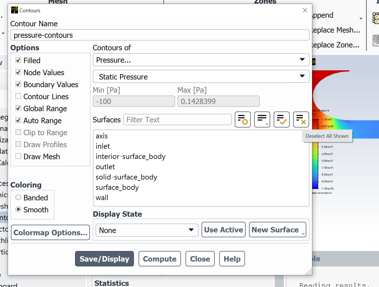
Step 11: Produce a pressure contour plot. In this step we will generate an image to show the distribution of pressure in the domain. Expand the Results and Graphics items on the Tree menu. Double click Contours to bring up Contours window. In the Contour Name box, enter the name "pressure-contours". Under Contours of, the default of Pressure and Static pressure should be selected. If not, select these from the drop down. Finally, deselect everything in the Surfaces list, by clicking the Deselect All Shown button or just clicking each surface one by one. Click the Save/Display button.
The window should display the pressure contours calculated inside the orifice plate, similar (but not necessarily identical) to the image above. If you can't see the picture, it might be because you need to select the tab at the top of the graphics window that says "Contours of Static Pressure [Pa]". You can also select the Scaled Residuals from the other tab. In the image, the red colour indicates high pressure, as illustrated on the scale to the left. The pressure at the end of the tube should be -100 Pa, as this was spcified as a boundary condition, and the pressure upstream will be around zero (gauge).
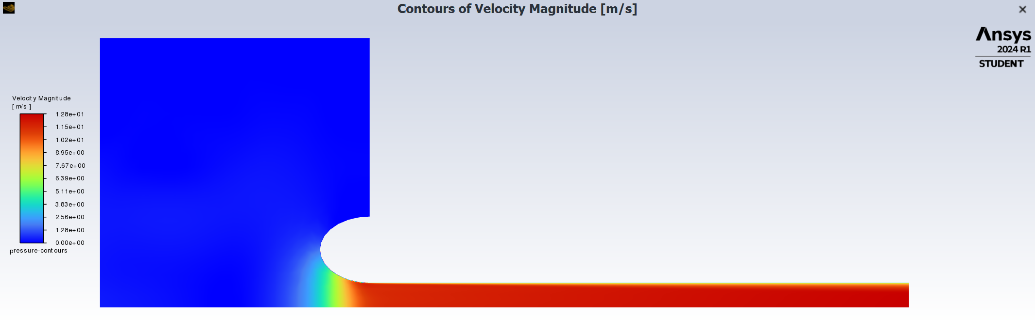
Step 12: Produce a velocity contour plot. In this step we will generate an image to show the distribution of velocity in the domain. Double click the Contours item from the tree menu again to bring up the Contours window. In the Contour Name box, enter the name "velocity-contours". Under Contours of, change the default to Velocity and Velocity Magnitude. Deselect everything in the Surfaces list, by clicking the Deselect All Shown button and click the Save/Display button.
The window should display the velocity contours in the Graphics window, with a scale in m/s to the left. You should be able to see the fluid accelerating as it is drawn into the bell mouth inlet.
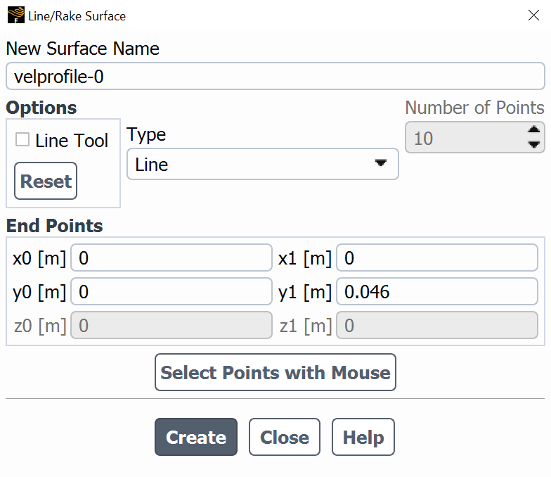
Step 13: Create a line. In this step, we will create a line in the domain so we can produce a graph in the next step. Using the menus at the top of the Fluent window, select Domain, Surface, +Create, and Line/Rake. Under "New Surface Name," enter the name velprofile-0 (or something else meaningful). The "End Points" allow you to specify two points on the X and Y coordinate system that define the start and end points of a line. To create a vertical line across the tube, directly after the curvature of the bell mouth, enter the following coordinates:
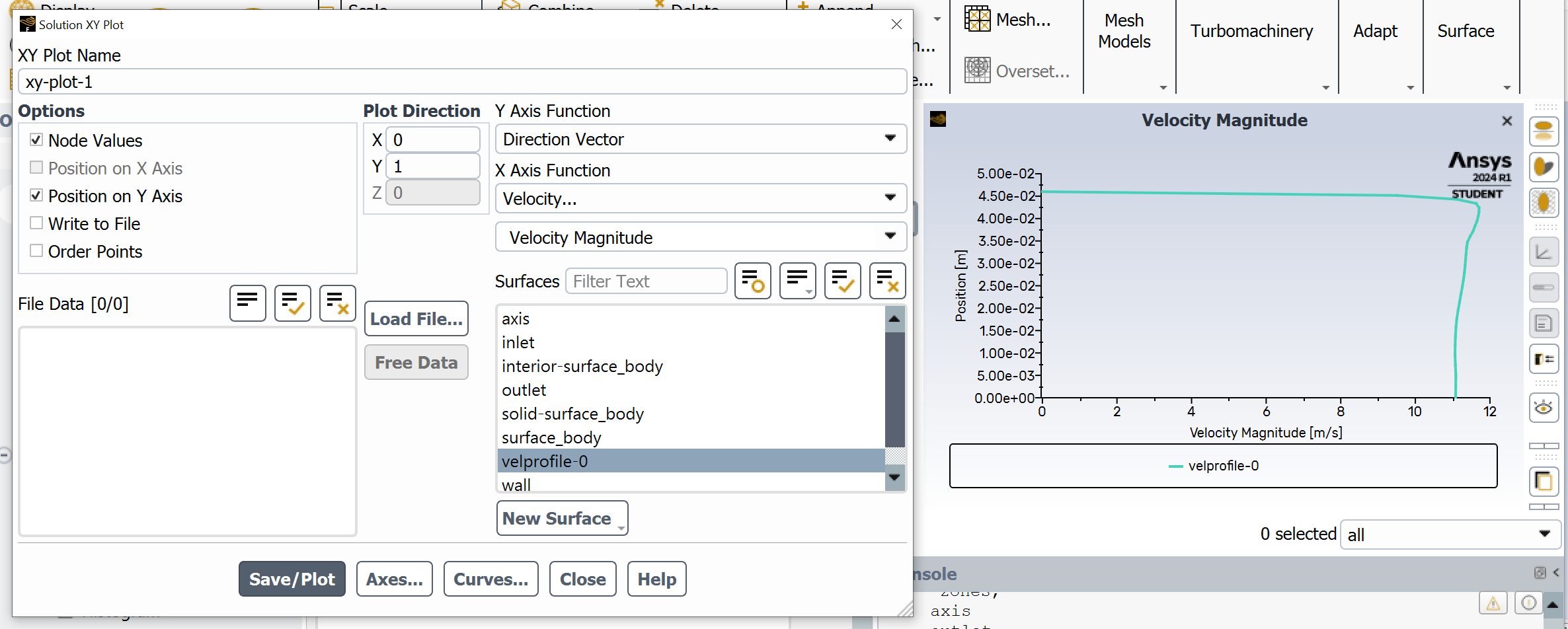
Step 15: Produce a graph of the velocity profile. In this step we will generate a graph of the pressure distribution along the axis. Expand the Results and Plots items on the Tree menu. Double click XY Plot to bring up Solution XY Plot window. Under XY Plot Name enter a meaningful name, such as "velocityprofile0". As we would like to create a plot that mirrors the distribution across the tube, we want the velocity plotted on the horizontal axis and the direction on the vertical axis. Under "Options" Deselect Position on X Axis and select Position on Y Axis. Change the Plot Direction as X=0, Y=1, as the axis is in the positive Y direction. In the dropdown menuse, set the X Axis Function to Velocity and Velocity Magnitude. Finally, select the newly created line velprofile-0 from the list of surfaces. Click the Save/Plot button and the graph of static pressure along the axis should appear in the Graphics window.
Step 16: Read data from the graph. Approximate data can be extracted by sight by reading the axes of the graph. More precise data can be found by hovering the mouse pointer over lines on the graph and recording the information displayed. In the example below, the mouse is hovered over a point displaying an X value of 11.6 (meters per second) and a Y value of 4.35e-2 (meters from the axis of the wind tunnel).

While not necessary at this stage, as the simulation is over, it is a good habit to get into saving your work as you go along. This can be done from the File menu at the top, and selecting Save Project.
Using the simulation result, the thickness of the boundary layer (the height from the wall at which the velocity stops rapidly changing) can be measured and compared with an empirical prediction.
Step 17: Create more velocity profiles. The profile previously created at X=0 is consistent with the end of the bellmouth and start of the straight tube. The flow may not have settled. To create more velocity profiles, create more lines by repeating the procedure above. For example, a profile at 250 mm downstream of the inlet, called "velprofile-250," could be created using the following points:
Step 18: Compare the boundary layer thickness. Use the graph to record the bulk, free stream velocity and boundary layer thickness at various locations downstream of the inlet. Remember the radius of the tube is 46 mm, and your graph will read distance from the axis. Find a suitable empirical equation that predicts the boundary layer thickness. To do this, you will need to calculate the Reynolds number of the flow inside the boundary layer. You can then compare empirical predictions with the thickness found using the numerical simulation.
Now that you are able to preprocess the simulation and validate the solution with theory, consider attempting to adjust the parameters of the simulation. Can you repeat this with different outlet pressures (e.g. -150 or -200 Pa)? This will generate different velocities inside the tube. How does this affect the boundary layer thickness? Do these results compare better or worse with empirical predictions? Remember! When you make changes to the simulation parameters, you will need to repeat the initialization and run the calculation again before the results stored in the computer will change.
Congratulations on reaching the end of this tutorial. In summary, you have learned to: